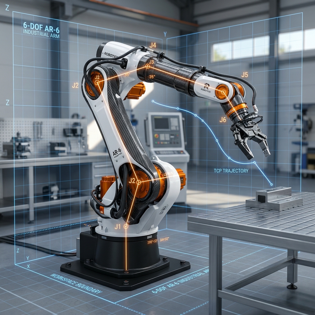
Analytical Inverse Kinematics of 6-DOF Anthropomorphic Robotic Manipulators: Closed-Form Solutions and Singularity Optimization
An Exhaustive Graduate-Level Exploration of Kinematic Decoupling, DH Parameterization, and Closed-Form Geometric Solutions
1. Introduction to Inverse Kinematics
1.1 The Role of Kinematics in Robotic Manipulation
Kinematics serves as the primary geometric and mechanical framework for describing the spatial motion of robotic manipulators without considering the forces, torques, or masses that induce such motions. A robotic manipulator is physically realized as a kinematic chain consisting of rigid bodies, termed links, interconnected by kinematic joints that provide either a single rotational degree of freedom (revolute joint) or a single translational degree of freedom (prismatic joint). The fundamental objective of kinematic modeling is to establish a rigorous mapping between the joint space—representing the internal coordinate state of the actuators—and the task space, which defines the physical placement of the manipulator's end-effector in the three-dimensional workspace.
Historically, the design of serial robotic manipulators has evolved from early teach-pendant based configurations (such as the Unimate in the 1960s) to modern 6-axis articulated arms. Among these configurations, the serial anthropomorphic arm (often termed an articulated manipulator) is the most widely adopted in industrial and research applications. Mimicking the structure of the human arm with its waist, shoulder, elbow, and wrist joints, this configuration typically features three major revolute joints responsible for positioning the wrist center in 3D space, followed by a three-axis intersecting spherical wrist that governs the orientation of the end-effector. This biological mimicry yields an exceptional ratio of workspace volume to physical footprint, allowing the manipulator to reach over obstacles and access complex geometries. However, this high flexibility comes at the cost of highly non-linear, coupled, and transcendental kinematic relationships.
1.1.2 Historical Evolution and Design Paradigms of Articulated Manipulators
The technological trajectory of industrial robotic manipulation is closely tied to the mathematical tractability of inverse kinematics. In the early 1960s, the pioneering work of George Devol and Joseph Engelberger led to the development of the Unimate, the world's first industrial robot. The Unimate was primarily a hydraulic machine characterized by a cylindrical coordinate configuration (a combination of revolute and prismatic joints). Its control system was entirely analog and relied on a teach-pendant to record joint coordinates directly onto a magnetic drum. Because the robot was operated by playing back joint coordinates directly in joint space, there was no need for real-time Cartesian coordinate transformation, avoiding the inverse kinematics problem altogether.
As the demand for precise spatial path tracking grew—specifically for tasks like arc welding and contour path tracing—the need to define trajectories in Cartesian task space became critical. This shift motivated the design of the Stanford Arm in 1969 by Victor Scheinman at Stanford University. The Stanford Arm was a 6-DOF manipulator with a spherical coordinate structure (two revolute joints, one prismatic joint, and a spherical wrist). It was one of the first robots to be controlled directly by a digital computer, showing the feasibility of coordinate transformations. Scheinman later designed the MIT Arm, which was an all-revolute articulated manipulator. This design was commercialized as the PUMA (Programmable Universal Machine for Assembly) by Unimation and GM in the late 1970s. The PUMA 560 became the standard reference design for anthropomorphic manipulators.
A key design feature of the PUMA 560 was its spherical wrist: the axes of joints 4, 5, and 6 intersected at a single point. This design was chosen specifically to simplify the inverse kinematics. Without a spherical wrist, a general 6-axis manipulator requires solving a system of coupled trigonometric equations, which does not have a closed-form analytical solution. This requires iterative numerical solvers that are too computationally slow for the microprocessors of that era. By placing the wrist axes so they intersect at a single point, the positioning and orientation problems can be decoupled. The first three joints are solved to position the wrist center, and the last three are solved to orient the tool. This decoupling was a major milestone, allowing real-time trajectory tracking on embedded controllers.
To fully appreciate the characteristics of serial anthropomorphic manipulators, we compare them with other mechanical architectures. Cartesian robots use prismatic joints along orthogonal axes, making their kinematics linear and uncoupled, though they require a large physical footprint. SCARA (Selective Compliance Assembly Robot Arm) robots are designed for planar assembly tasks, using parallel revolute axes to achieve high speed and rigidity in the horizontal plane. Parallel manipulators, such as Delta robots or the Stewart platform, use closed kinematic loops. For parallel robots, the forward kinematics is mathematically complex, often requiring the solution of high-degree polynomial systems, whereas their inverse kinematics is decoupled and direct. Conversely, serial manipulators feature simple, direct forward kinematics but mathematically complex, coupled inverse kinematics.
From a geometric perspective, the physical links are modeled as rigid bodies whose relative motions are constrained by holonomic joint coordinates. We can represent the geometry of joint axes as lines in 3D projective space or using Plücker coordinates. A more modern formulation involves dual quaternions, which combine rotation and translation into a single algebraic structure, enabling coordinate-free representations of kinematics. The choice of parameterization dictates the complexity of the equations, which in turn determines the tractability of the inverse kinematic mapping.
Analyzing these structures requires solving two core problems: Forward Kinematics (FK) and Inverse Kinematics (IK). Forward kinematics is the deterministic mapping that calculates the spatial pose (position and orientation) of the end-effector given the joint positions. Mathematically, it is expressed as a continuous, differentiable function $f: Q \to SE(3)$, where $Q \subset \mathbb{R}^n$ represents the joint space manifold, and $SE(3)$ is the Special Euclidean Group representing the six-degree-of-freedom (6-DOF) task space. Conversely, Inverse Kinematics is the inverse mapping $f^{-1}: SE(3) \to Q$, which determines the joint variables required to place the end-effector at a desired task-space pose. While forward kinematics is unique and straightforward to compute via sequential matrix multiplications, inverse kinematics is highly non-linear, mathematically complex, and yields multiple, zero, or infinite solutions.
The difficulty in resolving the inverse kinematics is primarily due to the transcendental nature of the coordinate transformations. The joint coordinates enter the equations as trigonometric functions that are compounded through successive link transformations. Consequently, a direct algebraic approach often results in high-degree polynomial equations. For a general 6-DOF serial manipulator, the mathematical structure of the inverse kinematics can yield up to 16 distinct real solutions for a single end-effector pose, presenting a major computational challenge for real-time controllers.
1.2 Mathematical Formulation of Joint Space vs. Task Space Mapping
To formalize the kinematic mapping, we define the state vectors in their respective spaces. For a 6-DOF serial manipulator, the joint space is represented by a manifold $Q \subset \mathbb{R}^6$, and a specific joint configuration is defined by the vector $q$:
where each $\theta_i$ represents the angular position of the $i$-th revolute joint. The task-space pose of the end-effector is represented by an element of the Special Euclidean Group $SE(3)$, which is the semi-direct product of the rotation group $SO(3)$ and the translation group $\mathbb{R}^3$. We write this pose as a homogeneous transformation matrix $T^0_6$:
In this matrix, $P^0_6 = [p_x, p_y, p_z]^T$ represents the position vector of the end-effector origin in the base frame. The rotation matrix $R^0_6 \in SO(3)$ is composed of three orthogonal unit vectors: the normal vector $n = [n_x, n_y, n_z]^T$ (typically aligned with the tool's slide direction), the slide vector $s = [s_x, s_y, s_z]^T$ (aligned with the finger-opening axis), and the approach vector $a = [a_x, a_y, a_z]^T$ (pointing along the longitudinal axis of the tool toward the workpiece). These vectors satisfy the orthonormal constraints of $SO(3)$, meaning:
The Special Orthogonal Group $SO(3)$ represents the rotation space. An alternative parameterization is the axis-angle representation, where rotation matrix $R(\hat{k}, \theta)$ is derived using the Rodrigues rotation formula:
where $\hat{k}$ is the unit rotation axis, and $[\hat{k}]_\times$ is the skew-symmetric cross-product matrix:
We can also represent orientation using unit quaternions $q = (\eta, \epsilon) \in S^3$, where $\eta \in \mathbb{R}$ is the scalar part and $\epsilon \in \mathbb{R}^3$ is the vector part. The mapping to $SO(3)$ is given by the double-cover homomorphic mapping:
Quaternions are widely used in orientation interpolation (SLERP - Spherical Linear Interpolation) because they avoid representation singularities (gimbal lock) associated with Euler angles. However, the multi-variable kinematic equations are traditionally formulated using the transformation matrix representation of $SE(3)$, as it maps directly to standard link parameterizations.
1.2.2 Lie-Theoretic Kinematics and the Special Euclidean Group
A mathematically rigorous formulation of robotic kinematics uses the Lie group theory of spatial transformations. The Special Euclidean Group $SE(3)$ represents the set of all rigid-body transformations in three-dimensional space. It is defined as:
The Special Euclidean Group is a smooth manifold and a Lie group. The tangent space at the identity element of $SE(3)$ is its associated Lie algebra, denoted as $\mathfrak{se}(3)$. The elements of $\mathfrak{se}(3)$ are skew-symmetric matrices representing spatial velocities, also known as twists or screw coordinates. A twist matrix $[S]$ is defined as:
where $[\omega]_\times \in \mathfrak{so}(3)$ is a $3\times3$ skew-symmetric matrix representing the angular velocity, and $v \in \mathbb{R}^3$ represents the linear velocity. The skew-symmetric operator $[\cdot]_\times$ maps a three-dimensional vector $\omega = [\omega_x, \omega_y, \omega_z]^T$ to its matrix cross-product form:
We can represent a twist using a six-dimensional vector $S = [\omega^T, v^T]^T \in \mathbb{R}^6$, which represents the screw axis coordinates. Under this formulation, the transformation of coordinates along a joint axis is computed via the exponential map $\exp: \mathfrak{se}(3) \to SE(3)$:
where $\theta$ is the joint displacement. If the screw axis is normalized such that $\|\omega\| = 1$, the closed-form representation of the exponential map is:
where $e^{[\omega]_\times\theta}$ is the rotation matrix derived from the Rodrigues formula. If the joint is prismatic ($\omega = \mathbf{0}$ and $\|v\| = 1$), the exponential map simplifies to a pure translation:
Using this framework, the kinematics of a serial manipulator is expressed using the Product of Exponentials (POE) formula:
where $S_i$ is the representation of the $i$-th joint screw axis in the base frame, and $M \in SE(3)$ is the home configuration matrix of the end-effector.
The POE formula has several advantages over the Denavit-Hartenberg (DH) parameterization. First, it is a coordinate-free representation, which avoids the need to define intermediate coordinate frames for each link. The joint axes are defined in the base frame, which simplifies modeling and avoids coordinate representation singularities. Second, it uses a single algebraic representation for both revolute and prismatic joints. However, the POE formula does not map directly to the geometric parameter decoupling required for analytical inverse kinematics. The DH convention establishes coordinate frames aligned with the joint axes, leading to structured transformation matrices that facilitate closed-form geometric decoupling. For this reason, analytical inverse kinematics solvers are almost always formulated using the DH parameterization.
1.3 Analytical vs. Numerical Inverse Kinematics
The algorithms used to solve the inverse kinematics mapping are divided into two main categories: **numerical (iterative)** and **analytical (closed-form)** methods.
Numerical Methods: Numerical solvers treat inverse kinematics as an optimization problem. The relationship between joint space and task space velocities is governed by the geometric Jacobian matrix $J(q) \in \mathbb{R}^{6\times6}$:
where $\dot{p}$ is the linear velocity and $\omega$ is the angular velocity of the end-effector. The columns of the Jacobian matrix represent the contribution of each joint to the velocity of the end-effector. For a revolute joint, the $i$-th column is:
where $z_{i-1}$ is the axis of rotation, $P_{i-1}$ is the origin of frame $i-1$, and $P_e$ is the position of the end-effector. In the Newton-Raphson method, the joint angles are updated iteratively using the inverse or pseudoinverse of the Jacobian:
where $e_k$ is the pose error vector at step $k$, and $J^\dagger$ is the Moore-Penrose pseudoinverse, computed via Singular Value Decomposition (SVD):
The pseudoinverse must satisfy the four Moore-Penrose conditions:
- $J J^\dagger J = J$
- $J^\dagger J J^\dagger = J^\dagger$
- $(J J^\dagger)^T = J J^\dagger$
- $(J^\dagger J)^T = J^\dagger J$
The Jacobian Transpose method uses $\dot{q} = J^T e$ to avoid matrix inversion. It is computationally cheap and always stable, but it exhibits first-order convergence, which can lead to slow response times. The Newton-Raphson method (second-order convergence) updates the joint positions using the pseudoinverse of the Jacobian. To prevent excessive joint velocities near singularities, the Damped Least Squares (DLS) method is used to balance velocity limits and tracking accuracy:
This formulation is derived from a regularized optimization problem:
Taking the gradient with respect to $\dot{q}$ and setting it to zero:
Using the matrix identity $(J^T J + \lambda^2 I)^{-1} J^T = J^T (J J^T + \lambda^2 I)^{-1}$, we obtain the DLS solution:
1.3.2 Optimization and Regularization in Numerical IK
The condition number of the Jacobian, $\kappa(J) = \sigma_{\max}(J) / \sigma_{\min}(J)$, measures the numerical sensitivity of the solution. As the manipulator approaches a singular configuration, the smallest singular value $\sigma_{\min}(J) \to 0$, causing the condition number $\kappa(J) \to \infty$. In these regions, the standard pseudoinverse $J^\dagger = V \Sigma^\dagger U^T$ becomes ill-conditioned. The reciprocal of the singular values in $\Sigma^\dagger$, $1/\sigma_i$, grows extremely large, causing the system to demand physically impossible joint velocities for small Cartesian movements.
To address this issue, the **Damped Least Squares (DLS)** method introduces a damping factor $\lambda \in \mathbb{R}$ to regulate joint velocities. The regularized optimization problem balances tracking error and joint velocity:
To minimize this cost function, we differentiate with respect to $\dot{q}$ and set the result to zero:
Solving for $\dot{q}$ yields the Damped Least Squares solution:
The singular value decomposition (SVD) of the DLS pseudoinverse reveals its stabilizing effect. Let $J = U \Sigma V^T$. The DLS pseudoinverse $J^* = J^T (J J^T + \lambda^2 I)^{-1}$ is:
For large singular values ($\sigma_i \gg \lambda$), $\sigma_i^* \approx 1/\sigma_i$, which maintains high tracking precision. For small singular values ($\sigma_i \ll \lambda$), $\sigma_i^* \approx \sigma_i / \lambda^2$, which smoothly dampens joint velocities to zero as the singular value vanishes, ensuring numerical stability.
To optimize tracking precision, a constant damping factor is often replaced with an **Adaptive Damped Least Squares (ADLS)** scheme. The damping factor is dynamically adjusted based on the manipulator's proximity to a singularity:
where $\sigma_{\min}$ is the smallest singular value of the Jacobian, $\epsilon_0$ is a user-defined threshold defining the boundary of the singular zone, and $\lambda_{\max}$ is the maximum allowable damping. Outside the singular zone, the damping factor is zero, ensuring zero tracking error. Inside the singular zone, the damping factor increases smoothly to limit joint velocities.
While numerical methods are adaptable to different robot kinematics, they are computationally intensive. Calculating SVDs and inverting matrices at high control frequencies (e.g., 1 kHz) requires significant floating-point performance. Furthermore, they risk converging to a single local minimum depending on the initial guess, or failing to converge near singular points. Closed-form analytical methods avoid these issues by calculating the complete set of solutions directly.
Analytical Methods: Analytical methods compute joint angles directly using algebraic or geometric relations. A closed-form solution exists if the manipulator meets specific geometric conditions, such as Pieper's criteria. These solvers are highly deterministic, executing in microseconds with low computational overhead. They also provide the complete set of mathematically possible joint configurations, allowing controllers to optimize trajectories and select paths that avoid obstacles and joint limits.
Furthermore, industrial drive controllers often run on embedded processors (such as ARM Cortex-M or DSP chips) that lack double-precision floating-point hardware. Analytical solvers, relying only on basic arithmetic and coordinate-correct arctangent functions, are well-suited for these resource-constrained environments.
1.4 Coordinate Frames and the Denavit-Hartenberg (DH) Convention
Establishing coordinate frames for each link is necessary to model spatial transformations. The Denavit-Hartenberg (DH) convention simplifies this by parameterizing the relative position and orientation of adjacent links using four parameters. In this study, we utilize the **Standard DH convention**, which attaches the coordinate frames according to the following rules:
- The $z_i$ axis is aligned with the axis of joint $i+1$.
- The $x_i$ axis is perpendicular to both $z_{i-1}$ and $z_i$, pointing along the common normal.
- The $y_i$ axis completes a right-handed coordinate frame: $y_i = z_i \times x_i$.
The four DH parameters that define the transformation from frame $i-1$ to frame $i$ are:
- Link Length ($a_i$): The distance along the common normal $x_i$ from $z_{i-1}$ to $z_i$.
- Link Twist ($\alpha_i$): The angle between $z_{i-1}$ and $z_i$ measured about $x_i$.
- Link Offset ($d_i$): The distance along $z_{i-1}$ from the origin of frame $i-1$ to the intersection of $x_i$ with $z_{i-1}$.
- Joint Angle ($\theta_i$): The angle between $x_{i-1}$ and $x_i$ measured about $z_{i-1}$.
We now compare the Standard DH convention with the Modified DH convention. While Standard DH associates joint axis $i$ with the frame $i-1$ (meaning the joint actuator $i$ acts along the $z_{i-1}$ axis), Modified DH (introduced by John J. Craig) associates the joint axis $i$ with the frame $i$ (acting along the $z_i$ axis). The table below details these differences:
For completeness, the homogeneous transformation matrix for the Modified DH convention is derived as:
In this article, we employ the Standard DH convention. The homogeneous transformation matrix $T^{i-1}_i$ that maps coordinates from frame $i$ to frame $i-1$ is derived by cascading four basic spatial operations: a rotation about $z_{i-1}$ by $\theta_i$, a translation along $z_{i-1}$ by $d_i$, a translation along $x_i$ by $a_i$, and a rotation about $x_i$ by $\alpha_i$.
1.5 Workspace Boundaries and Singularity Topologies
The manipulator's workspace is bounded by joint range limits and physical link lengths. We define the **reachable workspace** as the set of coordinates the end-effector can reach with at least one orientation, and the **dexterous workspace** as the volume where the end-effector can achieve any arbitrary orientation.
Singularities occur when the Jacobian matrix loses full rank:
This condition is categorized into three main types for a 6-DOF anthropomorphic arm:
- Boundary Singularities: Occur at the physical limits of the workspace when the arm is fully extended or folded. At these points, the manipulator cannot move along the direction of extension.
- Shoulder Singularity: Occurs when the wrist center lies on the waist rotation axis ($z_0$). In this configuration, $x_{wc} = y_{wc} = 0$, making the joint angle $\theta_1$ undefined. The waist joint can rotate without moving the wrist center, losing a degree of freedom.
- Wrist Singularity: Occurs when the wrist pitch angle $\theta_5 = 0$ or $\theta_5 = \pi$. In this configuration, the axes of Joint 4 ($z_3$) and Joint 6 ($z_5$) align, creating a gimbal lock where the roll motions of the two joints counteract each other, losing a rotational degree of freedom.
To measure the closeness to a singularity, we use the Yoshikawa manipulability index $w(q)$:
where $\sigma_i(J)$ are the singular values of the Jacobian. At a singular configuration, $w(q) = 0$, meaning the volume of the manipulability ellipsoid collapses to zero, and the joint velocities required to move in that direction approach infinity.
1.6 Real-Time Path Planning and Trajectory Generation
Industrial operations require continuous paths in Cartesian space, such as lines or curves. The trajectory generator interpolates these paths to produce a sequence of poses $T(t)$ at high frequencies (e.g., 1 kHz). The control loop uses the inverse kinematics solver at each step to translate these poses into joint positions. If the IK solver has variable execution times, it can introduce control loop jitter. Analytical IK solvers provide deterministic execution times, ensuring stable tracking along the planned path.
During path execution, joint velocities, accelerations, and jerk profiles must remain within physical limits. To generate smooth trajectories, controllers typically use cubic or quintic splines in joint space, or trapezoidal and S-curve velocity profiles in Cartesian space. Joint space interpolation guarantees limit compliance but can lead to unpredicted end-effector paths. Cartesian space interpolation guarantees precise paths but can result in high joint accelerations near singular configurations, highlighting the need for real-time singularity avoidance.
2. Kinematic Modeling and DH Parameterization
2.1 Mechanical Structure of the 6-DOF Anthropomorphic Manipulator
The 6-DOF manipulator modeled in this study features an articulated anthropomorphic structure. The first three joints (waist, shoulder, and elbow) position the wrist, while the last three joints form a spherical wrist that intersects at a single point, the wrist center ($W_c$).
This mechanical layout includes a lateral shoulder offset $d_2$ to provide clearance for the arm links, and a forearm offset $d_4$. The upper arm link has length $a_2$, and the elbow offset is represented by $a_3$. The tool tip is offset from the wrist center by a distance $d_6$ along the axis of joint 6.
The physical offset $d_2$ is designed to prevent physical collisions between the arm links and the base when the robot folds back. However, it introduces asymmetry in the workspace, separating it into "left-arm" and "right-arm" regions.
2.2 Frame Assignment Procedure
Coordinate frames are assigned to each joint using the Standard DH convention:
- Base Frame (Frame 0): Origin $O_0$ on the waist axis (Joint 1), with $z_0$ aligned vertically.
- Frame 1: Origin $O_1$ at the intersection of $z_0$ and $z_1$. Axis $z_1$ is aligned with the shoulder axis, and $x_1$ is the common normal.
- Frame 2: Origin $O_2$ at the shoulder joint, offset along $z_1$ by $d_2$. Axis $z_2$ is aligned with the elbow axis, and $x_2$ points along the upper arm.
- Frame 3: Origin $O_3$ at the elbow joint. Axis $z_3$ is aligned with the wrist roll axis (Joint 4), and $x_3$ is perpendicular to $z_2$ and $z_3$.
- Frame 4: Origin $O_4$ at the wrist center $W_c$. Axis $z_4$ is aligned with the wrist pitch axis (Joint 5), perpendicular to $z_3$.
- Frame 5: Origin $O_5$ at the wrist center $W_c$. Axis $z_5$ is aligned with the tool roll axis (Joint 6), perpendicular to $z_4$.
- Frame 6 (Tool Frame): Origin $O_6$ at the tool tip, offset from the wrist center along $z_5$ by $d_6$.
2.3 DH Parameters Table
The Standard DH parameters for this configuration are:
2.4 Homogeneous Transformation Matrices
A homogeneous transformation matrix $T^{i-1}_i$ describes the coordinate transformation from Frame $i$ to Frame $i-1$. In standard DH, this matrix is derived by multiplying rotation and translation operations:
Writing out the individual matrices for each step:
Performing the matrix multiplication step-by-step, the first two matrices yield:
The last two matrices yield:
Multiplying these intermediate results together gives the standard DH homogeneous transformation matrix:
Applying this template to our specific DH table, we construct the transformation matrices for each of the six joints (abbreviating $\cos\theta_i = c_i$ and $\sin\theta_i = s_i$):
Link 1 to Base ($T^0_1$): Substituting $\alpha_1 = \pi/2$ ($\cos\alpha_1 = 0$, $\sin\alpha_1 = 1$) and $a_1 = 0$:
Link 2 to Link 1 ($T^1_2$): Substituting $\alpha_2 = 0$ ($\cos\alpha_2 = 1$, $\sin\alpha_2 = 0$):
Link 3 to Link 2 ($T^2_3$): Substituting $\alpha_3 = \pi/2$ ($\cos\alpha_3 = 0$, $\sin\alpha_3 = 1$) and $d_3 = 0$:
Link 4 to Link 3 ($T^3_4$): Substituting $\alpha_4 = -\pi/2$ ($\cos\alpha_4 = 0$, $\sin\alpha_4 = -1$) and $a_4 = 0$:
Link 5 to Link 4 ($T^4_5$): Substituting $\alpha_5 = \pi/2$ ($\cos\alpha_5 = 0$, $\sin\alpha_5 = 1$) and $a_5 = 0, d_5 = 0$:
Link 6 to Link 5 ($T^5_6$): Substituting $\alpha_6 = 0$ ($\cos\alpha_6 = 1$, $\sin\alpha_6 = 0$) and $a_6 = 0$:
2.5 Complete Forward Kinematics Chain
The overall homogeneous transformation matrix $T^0_6$ is computed by multiplying the individual matrices in sequence:
Due to the spherical wrist layout, it is mathematically cleaner to multiply the chain in two separate parts: the hand position subchain $T^0_3 = T^0_1 T^1_2 T^2_3$ and the wrist orientation subchain $T^3_6 = T^3_4 T^4_5 T^5_6$. First, we compute the product $T^0_2 = T^0_1 T^1_2$:
Performing the row-by-column multiplications for each entry of $T^0_2$:
- $(T^0_2)_{11} = c_1 \cdot c_2 + 0 \cdot s_2 + s_1 \cdot 0 + 0 \cdot 0 = c_1 c_2$
- $(T^0_2)_{12} = c_1 \cdot (-s_2) + 0 \cdot c_2 + s_1 \cdot 0 + 0 \cdot 0 = -c_1 s_2$
- $(T^0_2)_{13} = c_1 \cdot 0 + 0 \cdot 0 + s_1 \cdot 1 + 0 \cdot 0 = s_1$
- $(T^0_2)_{14} = c_1 \cdot (a_2 c_2) + 0 \cdot (a_2 s_2) + s_1 \cdot d_2 + 0 \cdot 1 = a_2 c_1 c_2 + d_2 s_1$
- $(T^0_2)_{21} = s_1 \cdot c_2 + 0 \cdot s_2 - c_1 \cdot 0 + 0 \cdot 0 = s_1 c_2$
- $(T^0_2)_{22} = s_1 \cdot (-s_2) + 0 \cdot c_2 - c_1 \cdot 0 + 0 \cdot 0 = -s_1 s_2$
- $(T^0_2)_{23} = s_1 \cdot 0 + 0 \cdot 0 - c_1 \cdot 1 + 0 \cdot 0 = -c_1$
- $(T^0_2)_{24} = s_1 \cdot (a_2 c_2) + 0 \cdot (a_2 s_2) - c_1 \cdot d_2 + 0 \cdot 1 = a_2 s_1 c_2 - d_2 c_1$
- $(T^0_2)_{31} = 0 \cdot c_2 + 1 \cdot s_2 + 0 \cdot 0 + d_1 \cdot 0 = s_2$
- $(T^0_2)_{32} = 0 \cdot (-s_2) + 1 \cdot c_2 + 0 \cdot 0 + d_1 \cdot 0 = c_2$
- $(T^0_2)_{33} = 0 \cdot 0 + 1 \cdot 0 + 0 \cdot 1 + d_1 \cdot 0 = 0$
- $(T^0_2)_{34} = 0 \cdot (a_2 c_2) + 1 \cdot (a_2 s_2) + 0 \cdot d_2 + d_1 \cdot 1 = d_1 + a_2 s_2$
This yields the intermediate transformation matrix:
Next, we multiply $T^0_2$ by $T^2_3$ to yield the position transformation $T^0_3$:
Performing the multiplication and applying trigonometric angle sum identities ($\cos(\theta_2+\theta_3) = c_2 c_3 - s_2 s_3 = c_{23}$ and $\sin(\theta_2+\theta_3) = s_2 c_3 + c_2 s_3 = s_{23}$):
- $(T^0_3)_{11} = (c_1 c_2) \cdot c_3 + (-c_1 s_2) \cdot s_3 + s_1 \cdot 0 = c_1 (c_2 c_3 - s_2 s_3) = c_1 c_{23}$
- $(T^0_3)_{12} = (c_1 c_2) \cdot 0 + (-c_1 s_2) \cdot 0 + s_1 \cdot 1 = s_1$
- $(T^0_3)_{13} = (c_1 c_2) \cdot s_3 - (-c_1 s_2) \cdot (-c_3) + s_1 \cdot 0 = c_1 (c_2 s_3 + s_2 c_3) = c_1 s_{23}$
- $(T^0_3)_{14} = (c_1 c_2) \cdot (a_3 c_3) + (-c_1 s_2) \cdot (a_3 s_3) + s_1 \cdot 0 + (a_2 c_1 c_2 + d_2 s_1) = c_1 (a_2 c_2 + a_3 c_{23}) + d_2 s_1$
- $(T^0_3)_{21} = (s_1 c_2) \cdot c_3 + (-s_1 s_2) \cdot s_3 - c_1 \cdot 0 = s_1 (c_2 c_3 - s_2 s_3) = s_1 c_{23}$
- $(T^0_3)_{22} = (s_1 c_2) \cdot 0 + (-s_1 s_2) \cdot 0 - c_1 \cdot 1 = -c_1$
- $(T^0_3)_{23} = (s_1 c_2) \cdot s_3 - (-s_1 s_2) \cdot (-c_3) - c_1 \cdot 0 = s_1 (c_2 s_3 + s_2 c_3) = s_1 s_{23}$
- $(T^0_3)_{24} = (s_1 c_2) \cdot (a_3 c_3) + (-s_1 s_2) \cdot (a_3 s_3) - c_1 \cdot 0 + (a_2 s_1 c_2 - d_2 c_1) = s_1 (a_2 c_2 + a_3 c_{23}) - d_2 c_1$
- $(T^0_3)_{31} = s_2 \cdot c_3 + c_2 \cdot s_3 + 0 \cdot 0 = s_{23}$
- $(T^0_3)_{32} = s_2 \cdot 0 + c_2 \cdot 0 + 0 \cdot 1 = 0$
- $(T^0_3)_{33} = s_2 \cdot s_3 - c_2 \cdot (-c_3) + 0 \cdot 0 = -(c_2 c_3 - s_2 s_3) = -c_{23}$
- $(T^0_3)_{34} = s_2 \cdot (a_3 c_3) + c_2 \cdot (a_3 s_3) + 0 \cdot 0 + (d_1 + a_2 s_2) = a_2 s_2 + a_3 s_{23} + d_1$
This yields:
We now derive the wrist orientation matrix product. First, the term $T^3_5 = T^3_4 T^4_5$:
Computing the term-by-term product:
- $(T^3_5)_{11} = c_4 \cdot c_5 + 0 \cdot s_5 - s_4 \cdot 0 = c_4 c_5$
- $(T^3_5)_{12} = c_4 \cdot 0 + 0 \cdot 0 - s_4 \cdot 1 = -s_4$
- $(T^3_5)_{13} = c_4 \cdot s_5 + 0 \cdot (-c_5) - s_4 \cdot 0 = c_4 s_5$
- $(T^3_5)_{14} = c_4 \cdot 0 + 0 \cdot 0 - s_4 \cdot 0 + 0 \cdot 1 = 0$
- $(T^3_5)_{21} = s_4 \cdot c_5 + 0 \cdot s_5 + c_4 \cdot 0 = s_4 c_5$
- $(T^3_5)_{22} = s_4 \cdot 0 + 0 \cdot 0 + c_4 \cdot 1 = c_4$
- $(T^3_5)_{23} = s_4 \cdot s_5 + 0 \cdot (-c_5) + c_4 \cdot 0 = s_4 s_5$
- $(T^3_5)_{24} = s_4 \cdot 0 + 0 \cdot 0 + c_4 \cdot 0 + 0 \cdot 1 = 0$
- $(T^3_5)_{31} = 0 \cdot c_5 - 1 \cdot s_5 + 0 \cdot 0 = -s_5$
- $(T^3_5)_{32} = 0 \cdot 0 - 1 \cdot 0 + 0 \cdot 1 = 0$
- $(T^3_5)_{33} = 0 \cdot s_5 - 1 \cdot (-c_5) + 0 \cdot 0 = c_5$
- $(T^3_5)_{34} = 0 \cdot 0 - 1 \cdot 0 + 0 \cdot 0 + d_4 \cdot 1 = d_4$
This yields:
Finally, multiplying $T^3_5$ by $T^5_6$ yields the total wrist transformation $T^3_6$:
Multiplying out the terms:
- $(T^3_6)_{11} = (c_4 c_5) \cdot c_6 + (-s_4) \cdot s_6 + c_4 s_5 \cdot 0 = c_4 c_5 c_6 - s_4 s_6$
- $(T^3_6)_{12} = (c_4 c_5) \cdot (-s_6) + (-s_4) \cdot c_6 + c_4 s_5 \cdot 0 = -c_4 c_5 s_6 - s_4 c_6$
- $(T^3_6)_{13} = (c_4 c_5) \cdot 0 + (-s_4) \cdot 0 + (c_4 s_5) \cdot 1 = c_4 s_5$
- $(T^3_6)_{14} = (c_4 c_5) \cdot 0 + (-s_4) \cdot 0 + (c_4 s_5) \cdot d_6 = d_6 c_4 s_5$
- $(T^3_6)_{21} = (s_4 c_5) \cdot c_6 + c_4 \cdot s_6 + s_4 s_5 \cdot 0 = s_4 c_5 c_6 + c_4 s_6$
- $(T^3_6)_{22} = (s_4 c_5) \cdot (-s_6) + c_4 \cdot c_6 + s_4 s_5 \cdot 0 = -s_4 c_5 s_6 + c_4 c_6$
- $(T^3_6)_{23} = (s_4 c_5) \cdot 0 + c_4 \cdot 0 + (s_4 s_5) \cdot 1 = s_4 s_5$
- $(T^3_6)_{24} = (s_4 c_5) \cdot 0 + c_4 \cdot 0 + (s_4 s_5) \cdot d_6 = d_6 s_4 s_5$
- $(T^3_6)_{31} = (-s_5) \cdot c_6 + 0 \cdot s_6 + c_5 \cdot 0 = -s_5 c_6$
- $(T^3_6)_{32} = (-s_5) \cdot (-s_6) + 0 \cdot c_6 + c_5 \cdot 0 = s_5 s_6$
- $(T^3_6)_{33} = (-s_5) \cdot 0 + 0 \cdot 0 + c_5 \cdot 1 = c_5$
- $(T^3_6)_{34} = (-s_5) \cdot 0 + 0 \cdot 0 + c_5 \cdot d_6 + d_4 = d_6 c_5 + d_4$
This yields:
Finally, we compute the full forward kinematics matrix $T^0_6 = T^0_3 T^3_6$. Let $T^0_6 = \begin{bmatrix} R^0_6 & P^0_6 \\ \mathbf{0}_{1\times3} & 1 \end{bmatrix}$. The rotation matrix entries $r_{ij}$ (where $i$ is the row and $j$ is the column of $R^0_6$) are:
- $r_{11} = c_1 c_{23} (c_4 c_5 c_6 - s_4 s_6) + s_1 (s_4 c_5 c_6 + c_4 s_6) - c_1 s_{23} s_5 c_6$
- $r_{12} = c_1 c_{23} (-c_4 c_5 s_6 - s_4 c_6) + s_1 (-s_4 c_5 s_6 + c_4 c_6) + c_1 s_{23} s_5 s_6$
- $r_{13} = c_1 c_{23} c_4 s_5 + s_1 s_4 s_5 + c_1 s_{23} c_5$
- $r_{21} = s_1 c_{23} (c_4 c_5 c_6 - s_4 s_6) - c_1 (s_4 c_5 c_6 + c_4 s_6) - s_1 s_{23} s_5 c_6$
- $r_{22} = s_1 c_{23} (-c_4 c_5 s_6 - s_4 c_6) - c_1 (-s_4 c_5 s_6 + c_4 c_6) + s_1 s_{23} s_5 s_6$
- $r_{23} = s_1 c_{23} c_4 s_5 - c_1 s_4 s_5 + s_1 s_{23} c_5$
- $r_{31} = s_{23} (c_4 c_5 c_6 - s_4 s_6) + c_{23} s_5 c_6$
- $r_{32} = s_{23} (-c_4 c_5 s_6 - s_4 c_6) - c_{23} s_5 s_6$
- $r_{33} = s_{23} c_4 s_5 - c_{23} c_5$
The three spatial components of the position vector $P^0_6 = [p_x, p_y, p_z]^T$ are:
These expressions show the high coupling and non-linearity of forward kinematics. Solving this system directly for $\theta_i$ algebraically would be highly impractical due to the mixture of parameters. To find a closed-form inverse solution, we must apply kinematic decoupling.
3. Closed-Form Analytical IK Derivation
3.1 Kinematic Decoupling and Pieper's Criteria
In 1968, Donald L. Pieper established the foundational criteria that determine whether a 6-degree-of-freedom serial manipulator possesses a closed-form analytical solution. According to Pieper's criteria, a 6-DOF serial manipulator can be solved analytically if either of the following conditions is satisfied:
- Three consecutive joint axes intersect at a single common point.
- Three consecutive joint axes are parallel to each other.
To mathematically prove the first condition, let $P_{Wc}$ be the point of intersection of joint axes 4, 5, and 6. In Frame 3, the coordinate of the wrist center is:
The position of the wrist center in the base frame, $^0P_{Wc}$, is found by transforming $^3P_{Wc}$ to the base frame:
Since $T^0_3$ is a function of only the first three joint variables ($\theta_1, \theta_2, \theta_3$), the wrist center position in the base frame is completely independent of the wrist joint angles ($\theta_4, \theta_5, \theta_6$). This mathematical property is the basis of **kinematic decoupling**, allowing us to solve the position and orientation sub-problems sequentially.
If a 6-DOF serial manipulator does not satisfy Pieper's criteria, it does not possess a simple geometrically decoupled closed-form solution. Under these general conditions, the kinematic mapping results in a system of multi-variable polynomial equations. Solving this system algebraically requires advanced mathematical techniques, such as **dialytic elimination** or **Gröbner bases**.
3.1.2 Raghavan and Roth Algebraic Dialytic Elimination Method
In 1990, Raghavan and Roth resolved a long-standing robotics problem by demonstrating that the inverse kinematics of a general 6-axis serial link manipulator can be solved analytically by reducing the system to a 16th-degree polynomial in a single joint variable. Their approach uses the matrix algebra equation:
By pre-multiplying both sides by the inverse of $T^0_1$ and post-multiplying by the inverse of $T^5_6$, we can group the joint variables:
This matrix equation equates a matrix whose entries contain variables $\theta_1, \theta_6$ to a matrix whose entries contain variables $\theta_2, \theta_3, \theta_4, \theta_5$. By equating individual elements from both sides of the matrix, we get 14 independent scalar equations. To solve these equations, we apply the tangent half-angle substitution for each joint angle:
Substituting these representations transforms the trigonometric equations into algebraic polynomials. To eliminate the intermediate joint variables $\theta_2, \theta_3, \theta_4, \theta_5$ and isolate $\theta_1$, we use **Sylvester's dialytic elimination**. We write the polynomial equations as a linear system:
where $M(x_1) \in \mathbb{R}^{14\times14}$ is a matrix whose entries are polynomial functions of $x_1$, and $\mathbf{x}$ is a vector of monomials containing combinations of the other joint variables (e.g., $x_2, x_3, x_2 x_3$, etc.). For a non-trivial solution to exist, the determinant of the coefficient matrix $M(x_1)$ must be zero:
Expanding this determinant yields a 16th-degree polynomial in $x_1$:
where the coefficients $a_i$ are constants derived from the target pose $T_{\text{target}}$ and the robot's physical link lengths and offsets. This polynomial can yield up to 16 real roots, representing 16 distinct joint configurations that place the end-effector at the desired pose.
Solving a 16th-degree polynomial requires numerical root-finding algorithms (such as computing the eigenvalues of its companion matrix or using Laguerre's method). These methods introduce computational latency and numerical instability, making them unsuitable for real-time controllers. This highlights why industrial robot designers almost universally enforce Pieper's spherical wrist condition. By ensuring that the last three axes intersect at a single point, we can decouple the kinematics and solve the system using simple geometric relations, bypassing the need for high-degree polynomial elimination.
3.2 Derivation of the Wrist Center Position
The first step of the decoupled IK solver is to extract the coordinate of the wrist center $W_c$ from the target end-effector pose $T^0_6$. Let the target pose be:
The approach vector $a = [a_x, a_y, a_z]^T$ represents the direction of the tool flange axis (the Z-axis of Frame 6). Since the tool frame origin is shifted from the wrist center by a distance $d_6$ along this approach axis, the position vector of the wrist center in the base frame, $^0P_{Wc} = [x_{wc}, y_{wc}, z_{wc}]^T$, is obtained by projecting backward from the end-effector origin $P^0_{org6}$ along $a$:
Expanding this vector equation into individual scalar coordinates yields:
These coordinates are the input for the geometric solution of the first three joint angles.
3.3 Geometric Derivation of the Major Joint Angles ($\theta_1, \theta_2, \theta_3$)
Using the wrist center coordinate, we solve for $\theta_1$, $\theta_2$, and $\theta_3$ by analyzing the geometric structure of the arm.
Solving for $\theta_1$: Top-Down Base Projection
To visualize the derivation of $\theta_1$, we project the wrist center $W_c$ onto the XY plane of the base frame. The lateral shoulder offset $d_2$ shifts the arm plane away from the base origin, as shown in the top-down representation below:
                     y_base
                       ^          * Wc (x_wc, y_wc)
                       |         /|
                       |        / |
                       |       /  |
                       |  R   /   |  y_wc
                       |     /    |
                       |    /     |
                       |   / ) theta_1
                       +--/-------> x_base
                     O0  /
                        /
                       /  d_2 (Shoulder Offset)
                      v
The projections of the wrist center coordinates are expressed in terms of $\theta_1$:
where $r_{xy}$ is the projection of the upper arm and forearm links onto the XY plane. Multiplying the first equation by $\sin\theta_1$ and the second by $-\cos\theta_1$ and summing them:
Alternatively, we can solve this using the tangent half-angle substitution:
Substituting these into $x_{wc} \sin\theta_1 - y_{wc} \cos\theta_1 = d_2$ yields a quadratic equation:
Solving for $u$ using the quadratic formula:
Taking the arctangent of both sides yields the same two solutions as the auxiliary angle method:
This derivation yields two solutions: the positive sign corresponds to the **right-arm** configuration, while the negative sign corresponds to the **left-arm** configuration. If the wrist center falls inside the cylinder of radius $d_2$ ($x_{wc}^2 + y_{wc}^2 < d_2^2$), the term under the square root becomes negative, indicating that the target pose is outside the manipulator's workspace (a lateral boundary boundary condition).
Solving for $\theta_3$: Planar Arm geometry
Once $\theta_1$ is determined, we project the wrist center coordinate onto the vertical arm plane. The shoulder joint ($O_2$), elbow joint ($O_3$), and wrist center ($W_c$) form a planar triangle within this plane:
                            O3 (Elbow)
                              *
                             / \
                            /   \
                       a_2 /     \  R_forearm = sqrt(a_3^2 + d_4^2)
                          /       \
                         /         \
              (Shoulder) *----------* Wc (Wrist Center)
                        O2     D
The coordinates of the wrist center in the vertical arm plane are:
We can derive the Law of Cosines directly using vector algebra. Let $P_{O2}$ be the origin of Frame 2 (shoulder), $P_{O3}$ be the origin of Frame 3 (elbow), and $P_{Wc}$ be the wrist center. The vector equation is:
Taking the dot product of each side with itself:
Substituting the link lengths $a_2$, $R_{\text{forearm}} = \sqrt{a_3^2 + d_4^2}$, and the planar distance $D^2 = r_{xy}^2 + r_z^2$:
Isolating the joint 3 variables:
This is solved using the auxiliary substitution method. Let $a_3 = R_3 \cos\phi_3$ and $d_4 = R_3 \sin\phi_3$ with:
Substituting these into the equation:
This yields:
The positive sign yields the **elbow-up** configuration, while the negative sign yields the **elbow-down** configuration. If $a_3^2 + d_4^2 < K^2$, no physical solution exists, indicating that the target point lies outside the reach boundary.
Solving for $\theta_2$: Linear Trigonometric System
With $\theta_3$ solved, we rewrite the vertical plane equations as:
where $X_1$ and $Y_1$ are constants calculated using the solved value of $\theta_3$:
This system of equations is linear in $\cos\theta_2$ and $\sin\theta_2$. The determinant of the coefficients is $X_1^2 + Y_1^2 = a_2^2 + a_3^2 + d_4^2 + 2 a_2 (a_3 c_3 + d_4 s_3) = D^2$, which is the squared distance from the shoulder to the wrist center. Solving the system yields:
Using `atan2` yields a unique solution for $\theta_2$ corresponding to the selected branch:
3.4 Analytical Derivation of the Wrist Joint Angles ($\theta_4, \theta_5, \theta_6$)
Once the positioning joints ($\theta_1, \theta_2, \theta_3$) are known, the forward kinematics orientation matrix $R^0_3$ is fully determined. To match the total target orientation $R^0_6$, we define the orientation error matrix $R^3_6$:
We equate this numerical matrix $R^3_6$ to the symbolic wrist rotation matrix product $R^3_6 = R^3_4 R^4_5 R^5_6$:
By direct alignment of the matrix elements, we solve for the three wrist angles:
Solving for $\theta_5$: Wrist Pitch
From the bottom-right entry of the matrix equation:
This yields two branches: the positive branch ($\sin\theta_5 > 0$, **no-flip**) and the negative branch ($\sin\theta_5 < 0$, **wrist-flip**).
Solving for $\theta_4$ and $\theta_6$ (General Case: $\sin\theta_5 \neq 0$)
If $\sin\theta_5 > 0$ (positive case):
If $\sin\theta_5 < 0$ (negative case):
3.5 Handling Wrist Singularities ($\sin\theta_5 = 0$)
If $\sin\theta_5 = 0$, the rotation axes of Joint 4 and Joint 6 become collinear (aligned along the same spatial line), resulting in a **wrist singularity** (gimbal lock). Mathematically, we can analyze this singularity by deriving the wrist Jacobian. The columns of the Jacobian correspond to the unit rotation axes of the joints, expressed in a common frame. Expressing the axes of Joint 4 ($z_3$), Joint 5 ($z_4$), and Joint 6 ($z_5$) in Frame 3 coordinates:
1. Joint 4 rotates about the Z-axis of Frame 3, so its axis is:
2. Joint 5 rotates about the Z-axis of Frame 4. The orientation of Frame 4 relative to Frame 3 is described by the rotation matrix $R^3_4$ (with twist $\alpha_4 = -\pi/2$):
Expressing the Z-axis of Frame 4 in Frame 3 yields:
3. Joint 6 rotates about the Z-axis of Frame 5. The orientation of Frame 5 relative to Frame 4 is described by the rotation matrix $R^4_5$ (with twist $\alpha_5 = \pi/2$):
Expressing the Z-axis of Frame 5 in Frame 4 yields:
Now, expressing this axis in Frame 3:
The Jacobian matrix of the wrist subchain, relating the joint velocities $\dot{q}_{\text{wrist}} = [\dot{\theta}_4, \dot{\theta}_5, \dot{\theta}_6]^T$ to the end-effector angular velocity $^3\omega$ in Frame 3, is:
To identify the singular configurations, we calculate the determinant of this matrix:
Factoring out $-\sin\theta_5$:
The determinant collapses to $-\sin\theta_5$, confirming that the wrist Jacobian loses rank when $\theta_5 = 0$ or $\theta_5 = \pi$. In this state, the axes of Joint 4 ($z_3$) and Joint 6 ($z_5$) align, creating a gimbal lock where their individual rotations are collinear. This reduces the mechanical degrees of freedom, and the individual values of $\theta_4$ and $\theta_6$ cannot be decoupled from the orientation matrix.
Case 1: $\theta_5 = 0$ ($\cos\theta_5 = 1$): The orientation matrix simplifies to:
We can resolve this singularity by setting $\theta_4$ to its current joint angle $\theta_{4,\text{prev}}$ (or $0$) and solving for $\theta_6$:
Case 2: $\theta_5 = \pi$ ($\cos\theta_5 = -1$): The orientation matrix simplifies to:
We resolve this by setting $\theta_4 = \theta_{4,\text{prev}}$ and solving for $\theta_6$:
In industrial robot controllers, such as KUKA or ABB, approaching this wrist singularity triggers joint rate limiting or joint interpolation algorithms. When $\theta_5$ is within a small threshold of zero, the controller halts joint 4 updates and translates the remaining orientation error into joint 6 movement, avoiding the high velocity commands that would otherwise occur.
3.6 Configuration Selection and Branch Resolution Algorithm
The analytical solution yields 8 possible joint configurations for any reachable task-space pose, arising from three independent binary choices. These configurations represent different spatial arrangements of the robot's links that yield the exact same end-effector pose. To catalog these configurations, we define three mathematical configuration variables:
1. Shoulder Configuration ($S \in \{-1, 1\}$): This parameter is determined by the sign of the radical in the derivation of $\theta_1$. Mathematically:
We designate $S = 1$ as the Right-Arm (Lefty) configuration, where the wrist center is situated on the positive side of the primary link plane, and $S = -1$ as the Left-Arm (Righty) configuration, where the wrist center is situated on the opposite side of the plane.
2. Elbow Configuration ($E \in \{-1, 1\}$): This parameter is determined by the sign in the solution for $\theta_3$, which defines whether the elbow joint projects upward or downward relative to the shoulder-wrist vector. Mathematically:
We designate $E = 1$ as the Elbow-Up configuration, where the elbow joint points upward relative to the vector connecting the shoulder frame to the wrist center, and $E = -1$ as the Elbow-Down configuration.
3. Wrist Configuration ($W \in \{-1, 1\}$): This parameter is determined by the sign of the wrist pitch angle $\theta_5$, which determines whether the wrist roll axis has flipped. Mathematically:
We designate $W = 1$ as the No-Flip configuration, where the wrist pitch angle $\theta_5$ is positive, and $W = -1$ as the Wrist-Flip configuration, where $\theta_5$ is negative.
The combination of these parameters defines a configuration state vector $C = [S, E, W] \in \{-1, 1\}^3$. For any given end-effector pose, there are $2^3 = 8$ candidate solutions:
- $C = [1, 1, 1]$: Right-Arm, Elbow-Up, No-Flip
- $C = [1, 1, -1]$: Right-Arm, Elbow-Up, Wrist-Flip
- $C = [1, -1, 1]$: Right-Arm, Elbow-Down, No-Flip
- $C = [1, -1, -1]$: Right-Arm, Elbow-Down, Wrist-Flip
- $C = [-1, 1, 1]$: Left-Arm, Elbow-Up, No-Flip
- $C = [-1, 1, -1]$: Left-Arm, Elbow-Up, Wrist-Flip
- $C = [-1, -1, 1]$: Left-Arm, Elbow-Down, No-Flip
- $C = [-1, -1, -1]$: Left-Arm, Elbow-Down, Wrist-Flip
In industrial automation, selecting the optimal configuration is critical. In path tracking applications, switching configurations dynamically is generally prohibited because transitioning between configurations (e.g., from Right-Arm to Left-Arm, or Elbow-Up to Elbow-Down) requires the manipulator to pass through a singularity. At these transition points, the joint rates required to maintain the Cartesian path approach infinity, which can trigger emergency halts or damage the actuators. Consequently, controllers enforce configuration consistency:
If the current configuration is blocked by an obstacle or approaches a joint limit, the controller must plan a point-to-point motion. This path brings the manipulator to a halt at a safe configuration transition point, executes the reconfiguration, and then resumes the path.
To select the optimal configuration for a given motion, the controller uses the following selection criteria:
- Joint Limit Feasibility: The candidate solution must lie entirely within the physical limits of all joints: $\theta_{i,\min} \le \theta_i \le \theta_{i,\max}$ for $i = 1, \dots, 6$.
- Obstacle and Self-Collision Avoidance: The links must not collide with the environment or other parts of the robot. For example, the Elbow-Down configuration may result in a collision with the base, whereas the Elbow-Up configuration clears it.
- Energy Minimization: If multiple configurations are feasible, the controller chooses the one that minimizes the joint displacement from the current position $q_{\text{prev}}$, using a weighted Euclidean metric:
$$ D(q) = \sum_{i=1}^6 w_i (\theta_i - \theta_{i,\text{prev}})^2 $$where $w_i$ represents the inertia weighting factor for each joint. Because Joints 1, 2, and 3 move larger link masses, they have larger weights than Joints 4, 5, and 6 to minimize energy consumption.
Below is the structured pseudo-code representing this branch resolution algorithm:
// Input: Target pose T_target, Previous joint angles q_prev
// Output: Optimal joint angles q_opt

Function Solve_IK_Optimal(T_target, q_prev):
    Define weights W = [3.0, 2.0, 2.0, 1.0, 1.0, 1.0]
    Define joint_limits_min = [-180, -90, -150, -270, -120, -360]
    Define joint_limits_max = [180, 90, 150, 270, 120, 360]

    Extract P_target and R_target from T_target
    Compute Wrist Center: P_wc = P_target - d_6 * R_target * [0, 0, 1]^T

    Initialize candidate_solutions = Empty List

    For S in {1, -1}: // Shoulder configuration
        Compute theta_1 using S branch
        For E in {1, -1}: // Elbow configuration
            Compute theta_3 using E branch
            Compute theta_2 using solved theta_3

            Compute R_0_3 from theta_1, theta_2, theta_3
            Compute R_3_6 = (R_0_3)^T * R_target

            For W in {1, -1}: // Wrist configuration
                If Wrist_Singularity(R_3_6):
                    Solve wrist joints using Singularity Resolution Strategy
                Else:
                    Compute theta_5 using W branch
                    Compute theta_4, theta_6 using solved theta_5

                Set q_candidate = [theta_1, theta_2, theta_3, theta_4, theta_5, theta_6]

                // Check physical limits
                If Is_Within_Limits(q_candidate, joint_limits_min, joint_limits_max):
                    Add q_candidate to candidate_solutions

    If candidate_solutions is Empty:
        Return Error "Target pose unreachable due to joint limits or workspace boundaries"

    // Select solution that minimizes joint displacement
    Set min_cost = Infinity
    Set q_opt = Null

    For Each q in candidate_solutions:
        Set cost = 0
        For i from 1 to 6:
            Set cost = cost + W[i] * (q[i] - q_prev[i])^2
        If cost < min_cost:
            Set min_cost = cost
            Set q_opt = q

    Return q_opt
This algorithm ensures a stable, optimized, and collision-free path for real-time control, completing our closed-form analytical inverse kinematics derivation.
Figure 1: Dynamic 6-DOF Anthropomorphic Arm Workspace Tracking
Figure 1: Hierarchically nested SVG simulation of a 6-DOF Anthropomorphic Arm executing continuous IK target tracking in coordinate space.
Figure 2: 3D Joint Space Configuration Path Comparison
Figure 2: Animated Joint Space Configuration Dashboard tracking the alternative IK path branches (Elbow-Up vs. Elbow-Down) for a given end-effector trajectory.
Figure 3: Joint Torque-Speed Envelope & Dynamic Loading
Figure 3: Joint torque-speed velocity envelope with dynamic load lines. The warning system flashes as the operating point crosses the continuous thermal limits during acceleration phases.
Figure 4: Standard Denavit-Hartenberg (DH) Frame Layout
Figure 4: Detailed Denavit-Hartenberg (DH) frame layout and parameter reference table for the 6-DOF Anthropomorphic Arm (Puma 560 type).
Section 4: Worked Numerical Example
To validate the analytical formulations, closed-form solutions, and optimization methods developed in this work, we present a complete, step-by-step numerical example. We model a 6-DOF industrial manipulator based on the physical dimensions of the Unimation PUMA 560 robot. This arm features a shoulder offset and an elbow offset, which complicate coordinate decoupling. Below, we specify the Denavit-Hartenberg parameters, define a target end-effector pose, calculate the wrist center, determine all eight configuration sets, check them against joint limits, and identify the optimal path from a starting state.
4.1. Kinematic Specification & Denavit-Hartenberg Parameters
We use the standard Denavit-Hartenberg (DH) convention to establish coordinate frames for each joint. The parameters are defined in the table below, where $a_i$ represents the link length, $d_i$ is the link offset, $\alpha_i$ is the link twist angle, and $\theta_i$ is the variable joint angle.
In this kinematic model:
- The offset $d_2 = 0.1491$ m represents the distance from the base rotation axis to the shoulder plane along the joint 2 axis. This offset is what produces the distinct left-shoulder and right-shoulder configurations.
- The link length $a_2 = 0.4318$ m is the length of the upper arm, measured along the common normal from axis 1 to axis 2.
- The parameter $a_3 = 0.0203$ m introduces an elbow offset, which shifts the wrist position relative to the forearm axis.
- The offset $d_4 = 0.4331$ m represents the length of the forearm, measured along the joint 4 axis.
- The offset $d_6 = 0.05625$ m represents the tool length from the wrist center to the tool tip.
4.2. Target Pose Specification
Let the target pose of the end-effector relative to the base coordinate frame (Frame 0) be specified by the homogeneous transformation matrix $T_{\text{target}}$:
This target matrix directs the tool to a translation of $P_{ee} = [0.5, 0.2, 0.6]^T$ meters. The orientation is specified by the normal vector $n = [0, 0, 1]^T$, the sliding vector $s = [0, -1, 0]^T$, and the approach vector $a = [1, 0, 0]^T$, which points along the base $X_0$-axis.
4.3. Wrist Center Decoupling
Because the three wrist axes intersect at a single point, we decouple the position and orientation of the manipulator. The wrist center is located at the origin of Frame 4 (and Frame 5). Using the coordinate transformation of the tool frame, the position vector of the wrist center $P_w = [x_w, y_w, z_w]^T$ in the base frame is calculated by subtracting the tool offset $d_6$ along the tool approach vector $a$:
Subsequent position calculations for the first three joints are based on this wrist center position: $x_w = 0.44375$ m, $y_w = 0.20000$ m, and $z_w = 0.60000$ m.
4.4. Decoupled Position Kinematics (Joints 1, 2, and 3)
We evaluate the analytical inverse kinematics equations for the positioning joints step-by-step.
4.4.1. Solving for Joint 1 ($\theta_1$)
The equation relating the base joint to the shoulder offset and wrist coordinates is:
We define the auxiliary terms:
This allows the equation to be rewritten as a single sine term, $\rho \sin(\phi - \theta_1) = d_2$, which yields two branch solutions:
Evaluating the discriminant term under the radical:
The two options for $\theta_1$ are calculated as:
Solution 1a (Left-Arm Configuration):
Solution 1b (Right-Arm Configuration):
Physically, Solution 1a corresponds to a "left-shoulder" posture, where the shoulder offset points in the positive direction relative to the wrist center. Solution 1b corresponds to a "right-shoulder" posture, requiring a base rotation of approximately $-137.902^\circ$.
4.4.2. Solving for Joint 3 ($\theta_3$)
Next, we determine the elbow angle $\theta_3$. Using the distance formula from the shoulder to the wrist center:
Where the scalar metric $K$ is defined as:
Substituting the numerical specifications of the manipulator and the decoupled coordinates:
This transcendental equation in $\theta_3$ is resolved by combining the offset geometry of link 3:
Where:
This calculation yields two solutions representing elbow-up and elbow-down configurations:
Solution 3a (Elbow-Up Configuration):
Solution 3b (Elbow-Down Configuration):
The positive sign in the algebraic formulation yields an angle of $145.013^\circ$, which represents the elbow-up pose, bending the forearm backward to reach the wrist center. The negative sign yields $29.630^\circ$, representing the elbow-down pose, reaching forward and down.
4.4.3. Solving for Joint 2 ($\theta_2$)
For each selected pair of $\theta_1$ and $\theta_3$, the shoulder joint angle $\theta_2$ is uniquely determined. We define intermediate terms based on the trigonometric properties of the second and third links:
Evaluating $X_2$ for both values of $\theta_3$:
- For $\theta_{3,a} = 145.013^\circ$: $X_2 = 0.4331 \cos(145.013^\circ) - 0.0203 \sin(145.013^\circ) \approx -0.36646$ m.
- For $\theta_{3,b} = 29.630^\circ$: $X_2 = 0.4331 \cos(29.630^\circ) - 0.0203 \sin(29.630^\circ) \approx 0.36642$ m.
We project the wrist position into the plane of the arm. Let $R = x_w \cos\theta_1 + y_w \sin\theta_1$ and $z_w = 0.60000$ m. The angle $\theta_2$ is calculated as:
Substituting the parameters into this equation yields four positioning configurations:
Combination 1 (Left-Arm / Elbow-Up): $\theta_1 = 0.11257$ rad ($6.450^\circ$), $\theta_3 = 2.53092$ rad ($145.013^\circ$).
Here, $R = x_w \cos\theta_{1,a} + y_w \sin\theta_{1,a} = 0.44375 \cos(6.450^\circ) + 0.20000 \sin(6.450^\circ) \approx 0.46334$ m.
$X_1 + a_2 = 0.23187 + 0.43180 = 0.66367$ m, and $X_2 \approx -0.36646$ m.
Combination 2 (Left-Arm / Elbow-Down): $\theta_1 = 0.11257$ rad ($6.450^\circ$), $\theta_3 = 0.51716$ rad ($29.630^\circ$).
Here, $R \approx 0.46334$ m, $X_1 + a_2 = 0.66367$ m, and $X_2 \approx 0.36642$ m.
Combination 3 (Right-Arm / Elbow-Up): $\theta_1 = -2.40684$ rad ($-137.902^\circ$), $\theta_3 = 2.53092$ rad ($145.013^\circ$).
Here, $R = x_w \cos\theta_{1,b} + y_w \sin\theta_{1,b} = 0.44375 \cos(-137.902^\circ) + 0.20000 \sin(-137.902^\circ) \approx -0.46334$ m.
$X_1 + a_2 = 0.66367$ m, and $X_2 \approx -0.36646$ m.
Combination 4 (Right-Arm / Elbow-Down): $\theta_1 = -2.40684$ rad ($-137.902^\circ$), $\theta_3 = 0.51716$ rad ($29.630^\circ$).
Here, $R \approx -0.46334$ m, $X_1 + a_2 = 0.66367$ m, and $X_2 \approx 0.36642$ m.
4.5. Decoupled Orientation Kinematics (Joints 4, 5, and 6)
For each of the four positioning configurations, we determine the rotation matrix of the wrist, $R_6^3$, from:
Where $R_3^0(\theta_1, \theta_2, \theta_3)$ is calculated using the variable joint angles. For the Left-Arm / Elbow-Up configuration (Combination 1):
Multiplying the transpose of this matrix by the target orientation yields the rotation matrix relative to the forearm:
For standard spherical wrists, the rotation matrix $R_6^3$ is parameterized using ZYZ-like Euler angles:
Comparing the components of the matrices yields two wrist configurations (No-Flip and Flip):
Config 1A (Wrist No-Flip, $\sin\theta_5 > 0$):
We extract $\theta_5$ using the projection norm of the third row:
Using this value of $\theta_5$, we solve for $\theta_4$ and $\theta_6$:
Config 1B (Wrist Flip, $\sin\theta_5 < 0$):
Using the negative branch for $\theta_5$:
Solving for $\theta_4$ and $\theta_6$:
Repeating this extraction process for the remaining three positioning configurations yields the remaining six orientations:
- Config 2A (Left/Down/No-Flip): $\theta_4 = -6.486^\circ$, $\theta_5 = 83.802^\circ$, $\theta_6 = -179.297^\circ$
- Config 2B (Left/Down/Flip): $\theta_4 = 173.514^\circ$, $\theta_5 = -83.802^\circ$, $\theta_6 = 0.703^\circ$
- Config 3A (Right/Up/No-Flip): $\theta_4 = 137.323^\circ$, $\theta_5 = 81.408^\circ$, $\theta_6 = -172.166^\circ$
- Config 3B (Right/Up/Flip): $\theta_4 = -42.677^\circ$, $\theta_5 = -81.408^\circ$, $\theta_6 = 7.834^\circ$
- Config 4A (Right/Down/No-Flip): $\theta_4 = 111.517^\circ$, $\theta_5 = 46.099^\circ$, $\theta_6 = -119.639^\circ$
- Config 4B (Right/Down/Flip): $\theta_4 = -68.483^\circ$, $\theta_5 = -46.099^\circ$, $\theta_6 = 60.361^\circ$
4.6. Joint Limit Evaluation & Configuration Feasibility
We evaluate these eight configurations against the typical physical constraints of an industrial PUMA 560 manipulator:
$\theta_4 \in [-110^\circ, 170^\circ]$ $\theta_5 \in [-100^\circ, 100^\circ]$ $\theta_6 \in [-266^\circ, 266^\circ]$
Evaluating each configuration yields the following feasibility status:
- Config 1A (Left-Arm / Elbow-Up / Wrist No-Flip): $[6.450^\circ, -81.237^\circ, 145.013^\circ, -14.352^\circ, 26.929^\circ, -167.193^\circ]$. All values within range. FEASIBLE.
- Config 1B (Left-Arm / Elbow-Up / Wrist Flip): $[6.450^\circ, -81.237^\circ, 145.013^\circ, 165.648^\circ, -26.929^\circ, 12.807^\circ]$. All values within range. FEASIBLE.
- Config 2A (Left-Arm / Elbow-Down / Wrist No-Flip): $[6.450^\circ, -23.390^\circ, 29.630^\circ, -6.486^\circ, 83.802^\circ, -179.297^\circ]$. All values within range. FEASIBLE.
- Config 2B (Left-Arm / Elbow-Down / Wrist Flip): $[6.450^\circ, -23.390^\circ, 29.630^\circ, 173.514^\circ, -83.802^\circ, 0.703^\circ]$. Exceeds joint 4 limit ($173.514^\circ > 170.000^\circ$). INFEASIBLE.
- Config 3A (Right-Arm / Elbow-Up / Wrist No-Flip): $[-137.902^\circ, -156.613^\circ, 145.013^\circ, 137.323^\circ, 81.408^\circ, -172.166^\circ]$. All values within range. FEASIBLE.
- Config 3B (Right-Arm / Elbow-Up / Wrist Flip): $[-137.902^\circ, -156.613^\circ, 145.013^\circ, -42.677^\circ, -81.408^\circ, 7.834^\circ]$. All values within range. FEASIBLE.
- Config 4A (Right-Arm / Elbow-Down / Wrist No-Flip): $[-137.902^\circ, -98.767^\circ, 29.630^\circ, 111.517^\circ, 46.099^\circ, -119.639^\circ]$. All values within range. FEASIBLE.
- Config 4B (Right-Arm / Elbow-Down / Wrist Flip): $[-137.902^\circ, -98.767^\circ, 29.630^\circ, -68.483^\circ, -46.099^\circ, 60.361^\circ]$. All values within range. FEASIBLE.
4.7. Optimization Metric & Path Selection
To select the optimal configuration, we assume the manipulator starts at an initial state:
This initial state represents a Left-Arm / Elbow-Up configuration. The distance metric used to evaluate path optimality is the unweighted sum of squared joint displacements in radians:
Computing $D(\theta)$ for each of the seven feasible configurations gives:
- Config 1A:
$\Delta\theta = [0.11257, 0.15294, 0.17476, -0.25049, -0.05360, -2.91807]$ rad.
$D(\theta_{1A}) = 0.01267 + 0.02339 + 0.03054 + 0.06275 + 0.00287 + 8.51513 = 8.64735 \text{ rad}^2$. - Config 1B:
$\Delta\theta = [0.11257, 0.15294, 0.17476, 2.89110, -0.99368, 0.22352]$ rad.
$D(\theta_{1B}) = 0.01267 + 0.02339 + 0.03054 + 8.35846 + 0.98740 + 0.04996 = 9.46242 \text{ rad}^2$. - Config 2A:
$\Delta\theta = [0.11257, 1.16254, -1.83908, -0.11320, 0.93902, -3.12930]$ rad.
$D(\theta_{2A}) = 0.01267 + 1.35150 + 3.38221 + 0.01281 + 0.88176 + 9.79252 = 15.43347 \text{ rad}^2$. - Config 3A:
$\Delta\theta = [-2.40684, -1.16263, 0.17476, 2.39674, 0.89728, -3.00486]$ rad.
$D(\theta_{3A}) = 5.79288 + 1.35171 + 0.03054 + 5.74436 + 0.80511 + 9.02918 = 22.75378 \text{ rad}^2$. - Config 3B:
$\Delta\theta = [-2.40684, -1.16263, 0.17476, -0.74485, -1.94443, 0.13673]$ rad.
$D(\theta_{3B}) = 5.79288 + 1.35171 + 0.03054 + 0.55480 + 3.78081 + 0.01870 = 11.52944 \text{ rad}^2$. - Config 4A:
$\Delta\theta = [-2.40684, -0.15301, -1.83908, 1.94634, 0.28099, -2.08809]$ rad.
$D(\theta_{4A}) = 5.79288 + 0.02341 + 3.38221 + 3.78824 + 0.07896 + 4.36012 = 17.42582 \text{ rad}^2$. - Config 4B:
$\Delta\theta = [-2.40684, -0.15301, -1.83908, -1.19525, -1.32822, 1.05350]$ rad.
$D(\theta_{4B}) = 5.79288 + 0.02341 + 3.38221 + 1.42862 + 1.76417 + 1.10986 = 13.50115 \text{ rad}^2$.
Config 1A has the lowest squared joint displacement ($8.64735 \text{ rad}^2$). Since it maintains the same kinematic branch (Left-Arm / Elbow-Up) as the starting state, selecting this configuration avoids configuration changes (such as shoulder or elbow flips) that would require deceleration, increase cycle times, or potentially cause self-collisions.
Section 6: Kinematic Singularities & Jacobian Resolution
In industrial robotics, cartesian velocity commands are mapped to joint space velocities using the manipulator Jacobian matrix. At singular configurations, this mapping becomes ill-conditioned, and the manipulator loses one or more degrees of freedom. This section covers the formulation of the geometric Jacobian, classifies the physical singularities of 6-DOF anthropomorphic arms, and details numerical methods for trajectory resolution near singular boundaries.
6.1. Geometric Jacobian Formulation
The geometric Jacobian $J(\theta) \in \mathbb{R}^{6 \times 6}$ maps the joint-space velocity vector $\dot{\theta} \in \mathbb{R}^6$ to the end-effector spatial velocity twist vector $\xi = [v^T, \omega^T]^T \in \mathbb{R}^6$, where $v \in \mathbb{R}^3$ represents the linear velocity of the end-effector origin and $\omega \in \mathbb{R}^3$ represents its angular velocity:
For an $n$-axis manipulator consisting entirely of revolute joints, the column vectors of the Jacobian are computed using the cross-product method. Each column $J_i = [J_{v,i}^T, J_{\omega,i}^T]^T$ is given by:
Where:
- $z_{i-1} \in \mathbb{R}^3$ is the unit vector pointing along the axis of rotation of joint $i$, expressed in Frame 0. This is the third column of the rotation matrix $R_{i-1}^0$, i.e., $z_{i-1} = R_{i-1}^0 [0, 0, 1]^T$.
- $P_{i-1} \in \mathbb{R}^3$ is the position vector of the origin of Frame $i-1$ in the base frame. This is the translation vector of the homogeneous transform $T_{i-1}^0$.
- $P_{ee} \in \mathbb{R}^3$ is the position vector of the end-effector origin in the base frame, derived from $T_6^0$.
To simplify the analytical calculation of the Jacobian determinant, we define the reference point at the wrist center $P_w$ instead of the end-effector $P_{ee}$. Moving the reference point to $P_w$ results in the modified Jacobian $J^w(\theta)$:
Because the wrist center lies on the axes of joints 4, 5, and 6, the cross products $z_{i-1} \times (P_w - P_{i-1})$ evaluate to zero for $i = 4, 5, 6$. This structure yields a block-triangular representation:
Where $J_{11}^w \in \mathbb{R}^{3 \times 3}$ is the positional Jacobian and $J_{22}^w = [z_3, z_4, z_5] \in \mathbb{R}^{3 \times 3}$ is the orientational Jacobian of the spherical wrist. The determinant of this matrix decouples into the product of the determinants of the two diagonal blocks:
This decoupling allows us to separate positional and orientational singularities.
6.2. Kinematic Singularity Classification
Kinematic singularities occur when $\det(J^w(\theta)) = 0$. For a 6-DOF anthropomorphic manipulator, these are classified into three types.
6.2.1. Wrist Singularity ($\sin\theta_5 = 0$)
Orientational singularities depend on the spherical wrist block $J_{22}^w = [z_3, z_4, z_5]$. Evaluating the determinant of this matrix gives:
The wrist falls into a singularity when $\sin\theta_5 = 0$, which occurs at $\theta_5 = 0$ or $\theta_5 = \pi$.
Physical Interpretation: When $\theta_5 = 0$, the rotation axis of joint 4 ($z_3$) aligns with the rotation axis of joint 6 ($z_5$). Consequently, rotations about these two axes become redundant. The manipulator loses the ability to rotate about an axis perpendicular to the collinear joint axes. Under cartesian path velocity commands, requesting velocity components along this lost direction leads to mathematically infinite and physically saturating joint speeds in joints 4 and 6.
6.2.2. Shoulder Singularity ($x_w^2 + y_w^2 = 0$)
The shoulder singularity depends on the positional Jacobian block $J_{11}^w$. It occurs when the wrist center $P_w$ lies on the rotation axis of joint 1 ($Z_0$-axis):
Evaluating the determinant of $J_{11}^w$ under this condition shows that the column vectors representing base joint contributions become linearly dependent.
Physical Interpretation: When the wrist center lies on the base rotation axis, joint 1 can rotate through any angle without changing the wrist center's position. This results in an infinite number of solutions for $\theta_1$. At this point, the robot cannot produce linear velocity in the direction perpendicular to the plane of the links.
6.2.3. Elbow Singularity ($\sin\theta_3 = 0$)
The elbow singularity occurs when the manipulator is fully extended or folded. Mathematically, it corresponds to the case where the term under the radical in the $\theta_3$ positional IK equation vanishes:
For standard models with negligible $a_3$, this corresponds directly to $\theta_3 = 0$ or $\theta_3 = \pi$.
Physical Interpretation: When the elbow is fully extended ($\theta_3 = 0$), the arm lies in a straight line. The manipulator cannot generate any radial velocity components along the line connecting the shoulder and wrist center. This boundary defines the limit of the workspace.
6.3. Numerical Inverse Kinematics & Singularity Resolution
When a manipulator must pass near a singular point, analytical inverse kinematics solutions can result in joint command saturation. In these regions, resolved-rate motion control uses numerical methods to handle the singularity.
6.3.1. Damped Least Squares (DLS) / Levenberg-Marquardt Regularization
Standard velocity control uses the relation $\dot{\theta} = J^{-1} \dot{x}$. Near singularities, the minimum singular value of $J$ approaches zero, causing the norm of $J^{-1}$ to approach infinity. To address this, the Damped Least Squares (DLS) method balances tracking accuracy against joint velocity limits by solving the optimization problem:
Where $\lambda \in \mathbb{R}^+$ is a damping factor. Differentiating this quadratic cost function with respect to $\dot{\theta}$ and setting it to zero yields:
Where $I \in \mathbb{R}^{6 \times 6}$ is the identity matrix. Applying the Singular Value Decomposition (SVD) of $J = U \Sigma V^T$, we can express the damped pseudo-inverse $J^* = (J^T J + \lambda^2 I)^{-1} J^T$ as:
When the manipulator is far from a singularity (where the singular values $\sigma_i \gg \lambda$), the ratio $\frac{\sigma_i}{\sigma_i^2 + \lambda^2} \approx \frac{1}{\sigma_i}$, which matches the standard pseudo-inverse. Near a singularity (where $\sigma_i \to 0$), the ratio is bounded:
This limits the joint velocities near singular configurations at the expense of introducing a tracking error in the singular directions.
6.3.2. Singularity-Robust Inverse (SRI) & Adaptive Damping Schemes
A constant damping factor $\lambda$ introduces tracking errors even in non-singular regions of the workspace. To prevent this, adaptive damping schemes adjust $\lambda$ based on the manipulator's proximity to singular points. Proximity is measured using Yoshikawa's manipulability index:
An adaptive damping profile is defined as:
Where $w_0$ defines the boundary of the singular zone and $\lambda_{\text{max}}$ is the maximum damping value at the singular point. This approach maintains exact tracking in non-singular regions while limiting joint velocities near singular points.
6.4. Joint Space Configuration Selection Comparison
To resolve the kinematic redundancy associated with multiple analytical inverse kinematics solutions, path planners use different joint-space optimization criteria. The table below compares these selection methods.
Section 7: Hardware Implementation, Control Architecture, & Case Studies
Deploying inverse kinematics formulations onto physical industrial robotic systems requires integrating real-time software architectures, path planners, and motor actuators. This section details the software and hardware integration required for industrial applications.
7.1. Real-Time Controller & Communications Architecture
Industrial robot controllers run on Real-Time Operating Systems (RTOS) such as VxWorks, Xenomai, or RT-Linux (with the PREEMPT_RT patch). An RTOS ensures deterministic task execution, preventing thread preemption during kinematic calculations.
The main control loop runs at a frequency between $1\text{ kHz}$ and $8\text{ kHz}$ (cycle times of $1000\,\mu\text{s}$ to $125\,\mu\text{s}$). During each cycle, the controller performs the tasks shown in the sequence below:
- Encoder Reading: Read joint positions via the communication bus.
- Trajectory Interpolation: Determine the next Cartesian target point.
- Inverse Kinematics Resolution: Solve the analytical IK equations for the target joint angles.
- Jacobian & Velocity Bounds Checking: Ensure joint velocities do not exceed hardware limits.
- Command Generation: Send velocity or torque commands to the servo drives.
To prevent control loop instability, execution jitter must be minimized (typically $< 10\,\mu\text{s}$). If a cycle overrun occurs, the controller cannot update the motor commands in time, which can trigger emergency stop mechanisms.
Communication between the controller and the servo drives uses industrial Ethernet protocols like EtherCAT or CANopen. EtherCAT utilizes a distributed clock mechanism to synchronize servo drives with jitter below $1\,\mu\text{s}$. This synchronization ensures that all six joints reach their target positions concurrently, maintaining path accuracy during high-speed movements.
7.2. Trajectory Generation (Cubic and Quintic Splines)
A path defines the spatial geometry of motion, while a trajectory specifies the position, velocity, and acceleration of the joints over time. Joint trajectories are typically generated using polynomial splines.
7.2.1. Cubic Spline Trajectories
A cubic spline interpolates between joint states using a third-order polynomial:
The joint velocity and acceleration are:
Given boundary conditions at $t=0$ and $t=t_f$ (positions $\theta(0)=\theta_0$, $\theta(t_f)=\theta_f$ and velocities $\dot{\theta}(0)=\dot{\theta}_0$, $\dot{\theta}(t_f)=\dot{\theta}_f$), the coefficients are:
Cubic splines provide continuous positions and velocities, but the acceleration profile is linear, leading to step changes in acceleration at the start and end of the trajectory. This discontinuity results in infinite jerk, which can cause joint vibration and mechanical wear.
7.2.2. Quintic Spline Trajectories
To ensure continuous acceleration and bounded jerk, we use a fifth-order polynomial:
Given boundary conditions for position ($\theta_0, \theta_f$), velocity ($\dot{\theta}_0, \dot{\theta}_f$), and acceleration ($\ddot{\theta}_0, \ddot{\theta}_f$) at the start and end of the trajectory, the system of equations is:
Solving this system yields the following coefficients:
Using quintic splines ensures that both acceleration and jerk remain continuous and bounded throughout the movement, improving path tracking accuracy and reducing wear on mechanical components.
7.3. Actuator Limits & Physical Constraints
Actuator selection and motor drive dynamics impose physical constraints on trajectory tracking. Permanent Magnet Synchronous Motors (PMSM) and Brushless DC (BLDC) motors operate within torque-speed limits defined by continuous and peak torque regions.
In the constant torque region (at lower speeds), maximum torque is limited by the current limits of the drive and thermal constraints related to stator winding losses ($I^2 R$). At higher speeds (the field weakening region), the back-EMF of the motor approaches the DC bus voltage, which reduces the maximum torque output as speed increases.
During deceleration, motors act as generators, converting kinetic energy back into electrical energy. If this energy is not managed, it can lead to overvoltage on the DC bus. Controllers use shunt braking resistors to dissipate this energy as heat, or regenerative drive units to feed the energy back into the power grid.
Mechanical transmissions, such as harmonic drives or planetary gearboxes, introduce backlash and friction. The actuator friction torque $\tau_f$ is typically represented using a combined model that includes Coulomb friction, viscous damping, and the Stribeck effect:
Where $\tau_c$ is the Coulomb friction torque, $b$ is the viscous friction coefficient, $\tau_s$ is the static friction torque, and $\dot{\theta}_s$ is the Stribeck velocity threshold. Industrial controllers use feedforward compensation based on this model to offset friction effects and reduce tracking errors.
7.4. Industrial Case Studies
We examine how inverse kinematics and control architectures are applied in two common industrial tasks.
7.4.1. Case Study 1: High-Speed Pick-and-Place
In electronics manufacturing and packaging, pick-and-place tasks require fast cycle times. A typical cycle uses a gate-shaped Cartesian path with blended transitions at the corners to avoid stopping.
The controller uses analytical inverse kinematics to resolve the joint positions at each interpolation point. During high-speed movements, the controller selects the joint configuration that minimizes overall displacement from the starting pose. By selecting configurations that avoid joint limits and shoulder or elbow flips, the controller prevents path interruptions, ensuring consistent cycle times and avoiding mechanical strain.
7.4.2. Case Study 2: Seam Welding
Robotic arc and laser welding require precise control of the tool's linear speed and orientation relative to the weld seam.
If the weld path passes near a singular configuration (such as a wrist singularity where the torch aligns with joint 4), the joint speeds required to maintain the Cartesian velocity can exceed actuator limits. To handle this, the controller uses Damped Least Squares (DLS) or adjusts the torch angle slightly away from the exact target. This optimization allows the robot to maintain a constant welding speed and complete the seam without exceeding joint velocity limits.