Combustion DynamicsTurbulent FlamesLow-NOx CombustorsThermoacousticsChemical Kinetics30 min read

Advanced Combustion Dynamics & Low-NOx Combustors

An in-depth analysis of turbulent premixed combustion, chemical kinetics, and thermoacoustic instabilities in modern gas turbine systems. This technical guide covers key derivations, flame speed correlations, Rayleigh's criterion, and dry low-NOx design paradigms.

Advanced Combustion Dynamics & Low-NOx Combustors

Modern gas turbine combustion system design is driven by two competing constraints: the thermodynamic imperative for higher turbine inlet temperatures to maximize cycle efficiency, and stringent environmental regulations restricting emissions of nitrogen oxides ($NO_x$). The historical transition from conventional diffusion (non-premixed) combustors to Lean Premixed (LP) or Dry Low-$NO_x$ (DLN) systems represents a paradigm shift in combustion engineering. By premixing fuel and air upstream of the reaction zone and operating at equivalence ratios close to the lean limit, modern combustors achieve substantial emissions reductions. However, operating under these lean conditions introduces complex dynamics, including flame blowoff, flashback, and thermoacoustic instabilities. This article provides a rigorous analysis of turbulent premixed combustion, chemical kinetics, flame speed correlations, and the fundamental mechanics of thermoacoustic instabilities.

1. Turbulent Premixed Combustion Dynamics

Turbulent premixed combustion is characterized by the interaction of a chemical reaction zone with a turbulent flow field. Turbulence enhances the combustion rate by wrinkling the flame front, which increases the flame surface area and intensifies local heat and mass transfer. To describe these interactions mathematically, we consider the instantaneous governing equations of fluid motion and species transport. For a compressible, reactive flow, the local conservation of species mass fraction $Y_k$ and enthalpy $h$ are governed by:

$$ \frac{\partial (\rho Y_k)}{\partial t} + \nabla \cdot (\rho \vec{u} Y_k) = -\nabla \cdot \vec{J}_k + \dot{\omega}_k $$

where $\rho$ is the gas density, $\vec{u}$ is the velocity vector, $\vec{J}_k$ is the diffusion flux of species $k$ (often modeled using Fick's law as $\vec{J}_k = -\rho D_k \nabla Y_k$), and $\dot{\omega}_k$ is the net chemical production rate of species $k$. In turbulent flows, these variables are decomposed into mean and fluctuating components. Using Favre averaging (mass-weighted averaging) to handle density variations, we define:

$$ \tilde{\psi} = \frac{\overline{\rho \psi}}{\overline{\rho}} \quad \text{and} \quad \psi'' = \psi - \tilde{\psi} $$

Applying this decomposition to the species transport equation yields the Favre-averaged species equation:

$$ \frac{\partial (\bar{\rho} \tilde{Y}_k)}{\partial t} + \nabla \cdot (\bar{\rho} \tilde{\vec{u}} \tilde{Y}_k) = -\nabla \cdot \left( \overline{\vec{J}_k} + \bar{\rho} \widetilde{\vec{u}'' Y_k''} \right) + \overline{\dot{\omega}_k} $$

The term $\bar{\rho} \widetilde{\vec{u}'' Y_k''}$ represents turbulent transport (the scalar flux), which requires closure modeling (e.g., via the gradient diffusion hypothesis, $\bar{\rho} \widetilde{\vec{u}'' Y_k''} = -\bar{\rho} D_t \nabla \tilde{Y}_k$, where $D_t$ is the turbulent diffusivity). The term $\overline{\dot{\omega}_k}$ represents the mean chemical reaction rate, which is highly non-linear due to its Arrhenius temperature dependence and cannot be closed by simply evaluating the rate at mean temperatures and concentrations.

Regime Classification: The Borghi-Peters Diagram

The structure of a turbulent premixed flame is determined by the ratios of turbulent flow scales to chemical scales. The flow scales are defined by the integral length scale $l_0$ (representing the energy-containing eddies), the Kolmogorov length scale $\eta$ (representing the smallest dissipative eddies), and the turbulent fluctuation velocity $u'$. The chemical scales are defined by the laminar flame speed $S_L$ and the laminar flame thickness $\delta_L$, which is scaled as:

$$ \delta_L \approx \frac{D_{th}}{S_L} = \frac{\lambda}{\rho_u C_p S_L} $$

where $D_{th}$ is the thermal diffusivity, $\lambda$ is the thermal conductivity, and $\rho_u$ is the density of the unburned mixture. The interaction regimes are mapped on the Borghi-Peters diagram using three primary dimensionless parameters:

1. Turbulent Reynolds Number ($Re_t$): Represents the ratio of turbulent momentum transport to molecular viscous transport:

$$ Re_t = \frac{u' l_0}{\nu} \approx \frac{u' l_0}{S_L \delta_L} $$

2. Damköhler Number ($Da$): The ratio of the integral flow time scale $\tau_{flow} = l_0 / u'$ to the chemical reaction time scale $\tau_{chem} = \delta_L / S_L$:

$$ Da = \frac{\tau_{flow}}{\tau_{chem}} = \frac{l_0 S_L}{u' \delta_L} $$

3. Karlovitz Number ($Ka$): The ratio of the chemical time scale to the Kolmogorov time scale $\tau_\eta = (\nu/\epsilon)^{1/2}$, where $\epsilon$ is the kinetic energy dissipation rate:

$$ Ka = \frac{\tau_{chem}}{\tau_\eta} = \left(\frac{\delta_L}{\eta}\right)^2 $$

Using Kolmogorov relationships, namely $\eta/l_0 = Re_t^{-3/4}$ and $u_\eta/u' = Re_t^{-1/4}$, we can express the Karlovitz number as a function of the velocity and length scale ratios:

$$ Ka = \left( \frac{u'}{S_L} \right)^{3/2} \left( \frac{l_0}{\delta_L} \right)^{-1/2} $$

These relationships divide turbulent combustion into four distinct regimes on the Borghi-Peters diagram:

Wrinkled Flamelet Regime ($u' < S_L$ and $Ka < 1$): The flow fluctuations are too weak to wrinkle the flame front substantially. The flame maintains its laminar structure, and the local chemistry is identical to a one-dimensional laminar flame.
Corrugated Flamelet Regime ($u' > S_L$ and $Ka < 1$): The flame front is heavily folded and wrinkled by large turbulent eddies, forming pockets of reactants and products. However, because the Kolmogorov scale is larger than the flame thickness ($\eta > \delta_L$), the smallest eddies cannot enter the flame structure, leaving the internal thermal and species profiles of the flame sheet locally laminar.
Thin Reaction Zones ($Ka > 1$ and $Ka_\delta < 1$): The smallest eddies are smaller than the flame thickness ($\eta < \delta_L$) and can enter the preheat zone of the flame front, enhancing scalar transport. However, they are still larger than the inner reaction zone thickness ($\delta_r \approx 0.1 \delta_L$), meaning the chemical core of the flame remains unaffected by turbulence.
Broken Reaction Zones ($Ka_\delta > 1$): The smallest eddies ($\eta < \delta_r$) can enter the inner reaction zone, where they destroy the chemical structure of the flame by transporting reactants and heat away faster than the reactions can replenish them. This leads to localized flame quenching and distributed volumetric combustion.

Figure 1: Turbulent Premixed Flame Front Propagation and Swirl Stabilization

2. Chemical Kinetics & Arrhenius Reaction Rate Derivation

The macroscopic rate of chemical reactions is governed by the energy barrier that reactants must overcome to form products. We derive the Arrhenius equation using statistical thermodynamics and transition state theory. Consider the elementary bimolecular reaction:

$$ A + B \rightleftharpoons AB^\ddagger \rightarrow C + D $$

where $AB^\ddagger$ represents the activated complex (transition state). According to transition state theory, the reactants are in a state of quasi-equilibrium with the activated complex. The rate of the reaction is proportional to the concentration of the activated complex and the frequency of its passage over the activation energy barrier along the reaction coordinate:

$$ r = \nu^\ddagger [AB^\ddagger] $$

where $\nu^\ddagger$ is the vibrational frequency along the reaction coordinate. Using the classical statistical mechanics approximation, this frequency is given by:

$$ \nu^\ddagger = \frac{k_B T}{h} $$

where $k_B$ is Boltzmann's constant, $T$ is the temperature, and $h$ is Planck's constant. The equilibrium constant $K^\ddagger$ for the formation of the activated complex is defined as:

$$ K^\ddagger = \frac{[AB^\ddagger]}{[A][B]} $$

Thus, the reaction rate is:

$$ r = \frac{k_B T}{h} K^\ddagger [A][B] = k(T) [A][B] $$

where $k(T)$ is the temperature-dependent rate constant. Using the relation between the equilibrium constant and the Gibbs free energy of activation, $K^\ddagger = \exp(-\Delta G^\ddagger / R_u T)$, we write:

$$ k(T) = \frac{k_B T}{h} \exp\left( -\frac{\Delta G^\ddagger}{R_u T} \right) $$

Substituting $\Delta G^\ddagger = \Delta H^\ddagger - T \Delta S^\ddagger$, where $\Delta H^\ddagger$ is the enthalpy of activation and $\Delta S^\ddagger$ is the entropy of activation:

$$ k(T) = \left[ \frac{k_B T}{h} \exp\left( \frac{\Delta S^\ddagger}{R_u} \right) \right] \exp\left( -\frac{\Delta H^\ddagger}{R_u T} \right) $$

Approximating the enthalpy of activation $\Delta H^\ddagger$ as the activation energy $E_a$, and noting that the pre-exponential partition function terms can have a weak temperature dependence (modeled as $T^b$), we arrive at the modified Arrhenius equation:

$$ k(T) = A T^b \exp\left( -\frac{E_a}{R_u T} \right) $$

NOx Formation Kinetics

In gas turbine combustors, nitrogen oxides (primarily $NO$ and $NO_2$) are formed via several distinct pathways. The most prominent is the Thermal (Zeldovich) Mechanism, which dominant at high temperatures ($T > 1800$ K). The extended Zeldovich mechanism consists of three reversible reactions:

$ N_2 + O \overset{k_{1f}}{\underset{k_{1r}}{\rightleftharpoons}} NO + N $
$ N + O_2 \overset{k_{2f}}{\underset{k_{2r}}{\rightleftharpoons}} NO + O $
$ N + OH \overset{k_{3f}}{\underset{k_{3r}}{\rightleftharpoons}} NO + H $

The rates of change of $[NO]$ and $[N]$ concentrations are given by:

$$ \frac{d[NO]}{dt} = k_{1f}[N_2][O] - k_{1r}[NO][N] + k_{2f}[N][O_2] - k_{2r}[NO][O] + k_{3f}[N][OH] - k_{3r}[NO][H] $$

$$ \frac{d[N]}{dt} = k_{1f}[N_2][O] - k_{1r}[NO][N] - k_{2f}[N][O_2] + k_{2r}[NO][O] - k_{3f}[N][OH] + k_{3r}[NO][H] $$

Because the nitrogen radical $N$ is highly reactive, its concentration remains extremely low. Applying the Quasi-Steady State Assumption (QSSA) to $[N]$ (i.e., $d[N]/dt \approx 0$), we solve for the steady-state concentration $[N]_{ss}$:

$$ [N]_{ss} = \frac{k_{1f}[N_2][O] + k_{2r}[NO][O] + k_{3r}[NO][H]}{k_{1r}[NO] + k_{2f}[O_2] + k_{3f}[OH]} $$

Substituting $[N]_{ss}$ back into the rate equation for $[NO]$ yields the complete Zeldovich rate expression:

$$ \frac{d[NO]}{dt} = 2 k_{1f}[N_2][O] \frac{1 - \frac{[NO]^2}{K_{eq} [N_2][O_2]}}{1 + \frac{k_{1r}[NO]}{k_{2f}[O_2] + k_{3f}[OH]}} $$

where $K_{eq} = (k_{1f}k_{2f})/(k_{1r}k_{2r})$ is the equilibrium constant for the reaction $N_2 + O_2 \rightleftharpoons 2NO$. At early times or in lean flames where the $[NO]$ concentration is far below its equilibrium value ($[NO] \ll [NO]_{eq}$), the reverse reactions can be neglected, simplifying the rate equation to:

$$ \frac{d[NO]}{dt} \approx 2 k_{1f}[N_2][O] $$

This rate depends heavily on the concentration of oxygen atoms $[O]$. Assuming local thermodynamic equilibrium for the dissociation $O_2 \rightleftharpoons 2O$, the concentration is given by:

$$ [O] = K_O^{0.5} [O_2]^{0.5} $$

Because reaction (1) has a high activation energy ($E_{a,1} \approx 318$ kJ/mol), the rate constant $k_{1f}$ is highly sensitive to temperature. Therefore, thermal $NO_x$ formation increases exponentially with the flame temperature, which is the primary motivation for operating lean premixed combustors.

Other pathways include the Prompt (Fenimore) Mechanism, initiated by hydrocarbon radicals (e.g., $CH + N_2 \rightleftharpoons HCN + N$) in the flame front; the $N_2O$ Intermediate Pathway, which is important in lean, high-pressure systems; and the NNH Mechanism, which plays a role in hydrogen-rich flames.

3. Flame Speed Correlations

The laminar flame speed $S_L$ is a fundamental physicochemical property of a reactive mixture. It is defined as the velocity at which a planar, laminar, one-dimensional flame propagates relative to the unburned mixture. For methane-air mixtures, the laminar flame speed varies with equivalence ratio $\phi$, unburned gas temperature $T_u$, and pressure $P$. A widely used empirical correlation (Metghalchi and Keck) is:

$$ S_L(\phi, T_u, P) = S_{L,0}(\phi) \left( \frac{T_u}{T_0} \right)^\alpha \left( \frac{P}{P_0} \right)^\beta $$

where reference conditions are $T_0 = 298$ K and $P_0 = 0.1$ MPa. For methane, the reference speed is often modeled as:

$$ S_{L,0}(\phi) = w_1 + w_2 (\phi - \phi_{max})^2 $$

where $\phi_{max} \approx 1.08$, $w_1 \approx 0.38$ m/s, and $w_2 \approx -1.3$ m/s. The exponents $\alpha$ and $\beta$ account for the temperature and pressure dependence:

$$ \alpha = 2.18 - 0.8(\phi - 1) \quad \text{and} \quad \beta = -0.16 + 0.22(\phi - 1) $$

Note that $\beta$ is negative, indicating that $S_L$ decreases as pressure increases, which is typical for hydrocarbon flames due to the pressure-dependent radical recombination rates that limit the concentration of chain-branching radicals.

In turbulent flows, the flame is wrinkled, and the burning velocity increases to the turbulent flame speed $S_T$. The turbulent flame speed is modeled by balancing the area increase of the wrinkled flame sheet with the turbulent velocity fluctuations $u'$. In the corrugated flamelet regime, Damköhler proposed:

$$ \frac{S_T}{S_L} = 1 + C \frac{u'}{S_L} $$

where $C$ is an empirical constant of order unity. In the thin reaction zone regime, where smaller eddies penetrate the flame's preheat zone, the scaling becomes non-linear. Modern correlations based on renormalization group theory and G-equation formulations utilize a power-law relationship:

$$ \frac{S_T}{S_L} = 1 + C \left( \frac{u'}{S_L} \right)^n $$

where the exponent $n$ typically ranges between 0.7 and 0.85, representing a bending effect where the rate of increase of $S_T/S_L$ decreases at high turbulence intensities due to localized flame stretch and extinction.

4. Thermoacoustic Instabilities & Rayleigh Criterion Derivation

Thermoacoustic instability occurs when pressure oscillations in the combustion chamber couple with heat release rate oscillations of the flame. This coupling creates a self-excited feedback loop that can grow to high amplitudes. We derive the governing acoustic energy equation starting from the linearized, inviscid Euler equations with a heat source term.

The linearized momentum and energy equations for the acoustic perturbations are:

$$ \rho_0 \frac{\partial \vec{u}'}{\partial t} + \nabla p' = 0 $$

$$ \frac{\partial p'}{\partial t} - c_0^2 \frac{\partial \rho'}{\partial t} = (\gamma - 1) q' $$

where $p'$, $\vec{u}'$, $\rho'$, and $q'$ are the acoustic pressure, acoustic velocity vector, density perturbation, and heat release rate fluctuation per unit volume, respectively. The parameter $c_0$ is the speed of sound, $\rho_0$ is the mean density, and $\gamma$ is the ratio of specific heats.

First, we multiply the linearized momentum equation by the acoustic velocity $\vec{u}'$:

$$ \rho_0 \vec{u}' \cdot \frac{\partial \vec{u}'}{\partial t} + \vec{u}' \cdot \nabla p' = 0 \implies \frac{\partial}{\partial t} \left( \frac{1}{2} \rho_0 |\vec{u}'|^2 \right) + \vec{u}' \cdot \nabla p' = 0 $$

Next, we divide the energy equation by $\rho_0 c_0^2$ and multiply by the acoustic pressure $p'$:

$$ \frac{p'}{\rho_0 c_0^2} \frac{\partial p'}{\partial t} - \frac{p'}{\rho_0} \frac{\partial \rho'}{\partial t} = \frac{\gamma - 1}{\rho_0 c_0^2} p' q' $$

From the linearized continuity equation, we have $\partial \rho' / \partial t = -\rho_0 \nabla \cdot \vec{u}'$. Substituting this into the energy relation yields:

$$ \frac{\partial}{\partial t} \left( \frac{1}{2} \frac{p'^2}{\rho_0 c_0^2} \right) + p' \nabla \cdot \vec{u}' = \frac{\gamma - 1}{\rho_0 c_0^2} p' q' $$

Adding the kinetic energy and potential energy equations:

$$ \frac{\partial}{\partial t} \left( \frac{1}{2} \rho_0 |\vec{u}'|^2 + \frac{1}{2} \frac{p'^2}{\rho_0 c_0^2} \right) + \vec{u}' \cdot \nabla p' + p' \nabla \cdot \vec{u}' = \frac{\gamma - 1}{\rho_0 c_0^2} p' q' $$

Using the vector identity $\nabla \cdot (p' \vec{u}') = \vec{u}' \cdot \nabla p' + p' \nabla \cdot \vec{u}'$, we define the acoustic energy density $E_{ac}$ and acoustic energy flux $\vec{I}_{ac}$ as:

$$ E_{ac} = \frac{1}{2} \rho_0 |\vec{u}'|^2 + \frac{1}{2} \frac{p'^2}{\rho_0 c_0^2} \quad \text{and} \quad \vec{I}_{ac} = p' \vec{u}' $$

Substituting these definitions, and introducing a dissipation term $-\mathcal{D}$ to account for viscous effects, thermal boundary losses, and acoustic liners:

$$ \frac{\partial E_{ac}}{\partial t} + \nabla \cdot \vec{I}_{ac} = \frac{\gamma - 1}{\rho_0 c_0^2} p' q' - \mathcal{D} $$

Integrating this equation over a control volume $V$ representing the combustor, and integrating over a cycle period $T = 2\pi / \omega$ of the acoustic oscillation:

$$ \int_0^T \frac{d}{dt} \left( \int_V E_{ac} dV \right) dt + \int_0^T \oint_{\partial V} (p' \vec{u}') \cdot \hat{n} \, dS \, dt = \frac{\gamma - 1}{\rho_0 c_0^2} \int_0^T \int_V p'(x, t) q'(x, t) \, dV \, dt - \int_0^T \int_V \mathcal{D} \, dV \, dt $$

For a periodic instability, the system's energy returns to its initial value at the end of each cycle, meaning the first integral on the left side vanishes. We define the total energy losses per cycle as:

$$ \mathcal{L} = \int_0^T \oint_{\partial V} (p' \vec{u}') \cdot \hat{n} \, dS \, dt + \int_0^T \int_V \mathcal{D} \, dV \, dt $$

For the acoustic energy to grow (driving the instability), the driving term must exceed the losses. This yields the mathematical statement of the **Rayleigh Criterion**:

$$ \int_0^T \int_V p'(x, t) q'(x, t) \, dV \, dt > \mathcal{L} $$

Physically, the Rayleigh criterion states that acoustic energy is added to the system if the heat release rate fluctuations $q'$ are in phase with the acoustic pressure oscillations $p'$. If we write the oscillations as:

$$ p'(t) = P'_{amp} \cos(\omega t) \quad \text{and} \quad q'(t) = Q'_{amp} \cos(\omega t - \theta) $$

where $\theta$ is the phase difference between pressure and heat release. The cycle-integrated product is:

$$ \int_0^T p'(t) q'(t) dt = \frac{1}{2} P'_{amp} Q'_{amp} T \cos(\theta) $$

For the integral to be positive, we require $\cos(\theta) > 0$, which corresponds to:

$$ -\frac{\pi}{2} < \theta < \frac{\pi}{2} $$

This demonstrates that instabilities grow when the time delay between pressure and heat release fluctuations is short enough that they remain in phase. In gas turbines, this time delay is related to the convective transport time of fuel from the injector to the flame zone, leading to the classic $n-\tau$ model: $q'(t) = n \cdot u'(t - \tau)$, where $n$ is the interaction index and $\tau$ is the convective time delay.

Figure 2: Thermoacoustic Feedback Loop and Rayleigh Criterion (In-Phase vs Out-of-Phase Coupling)

5. Combustor Design & Instability Visualization

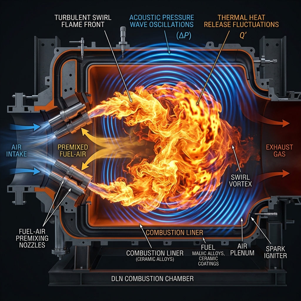
To visualize these coupled dynamics, the inline diagram below illustrates a typical Dry Low-$NO_x$ (DLN) swirl-stabilized combustor chamber. It highlights the main components, including the fuel-air premixing nozzle, the swiler vanes, the Central Recirculation Zone (CRZ) that stabilizes the flame, and the overlapping acoustic pressure waves and heat release fluctuations that drive thermoacoustic instabilities.

Figure 3: Dry Low-NOx (DLN) Combustor Swirl Stabilized Flame and Axial Temperature Profile

6. Comparative Analysis of Combustor Concepts

Combustor architectures are designed to balance emissions reduction, flame stability, and pressure drop. Below is a comparative technical analysis of five core combustor concepts used in utility and aviation gas turbines:

Combustor Concept	Equivalence Ratio Range ($\phi$)	NOx Emissions (ppm)	Thermoacoustic Vulnerability	Flashback/Blowout Risk	Key Stabilization Mechanism
Conventional Diffusion	0.8 - 1.2 (Local $\phi \approx 1.0$)	100 - 300	Very Low (Aerodynamically Damped)	None (No upstream premixing)	Shear layer mixing, pilot flame
Wet Low-NOx (Steam Inj.)	0.7 - 1.1	25 - 42	Low to Moderate	None (No upstream premixing)	Thermal diluent injection
Dry Low-NOx (DLN)	0.5 - 0.65	9 - 25	High (Highly susceptible)	High ( CIVB and boundary layers)	Swirl-induced vortex breakdown (CRZ)
Rich-Quench-Lean (RQL)	1.2 - 1.6 (Rich) to 0.4 - 0.6 (Lean)	20 - 50	Moderate	Low	Rapid mixing air jets, stage staging
Catalytic Combustors	0.3 - 0.5	< 3	Very Low	Moderate (substrate preheating)	Heterogeneous surface reaction

7. Worked Numerical Example

Problem Statement:

A lean-premixed gas turbine combustor operates on gaseous methane ($CH_4$) and air. The inlet conditions are:

Equivalence ratio: $\phi = 0.60$
Inlet temperature: $T_u = 650$ K
Combustor pressure: $P = 1.5$ MPa (15.0 bar)
Combustor residence time: $\tau = 8.0$ ms ($8.0 \times 10^{-3}$ s)

Calculate:

The adiabatic flame temperature $T_{ad}$ of the mixture. (Assume the lower heating value of methane is $LHV = 50.0 \times 10^3$ kJ/kg-fuel and the average specific heat of the product mixture is $C_{p,prod} = 1.25$ kJ/kg-K).
The thermal $NO$ formation rate $d[NO]/dt$ in mol/cm³-s at $T_{ad}$, using the simplified Zeldovich mechanism rate equation.
The total mass concentration of $NO$ produced over the residence time $\tau$, and the resulting Emission Index $EI_{NO}$ in g of $NO$ per kg of fuel.

Given Kinetic Data:

Rate constant $k_{1f} = 1.8 \times 10^{14} \exp\left(-\frac{38370}{T}\right)$ cm³/mol-s.
Equilibrium oxygen atom concentration is given by the empirical relation: $[O]_{eq} = 36.0 \cdot [O_2]_{eq}^{0.5} \exp\left(-\frac{27000}{T}\right)$ mol/cm³.

Solution Step-by-Step

Step 1: Calculate the adiabatic flame temperature ($T_{ad}$)

First, we write the stoichiometric reaction for methane and air:

$$ CH_4 + 2 (O_2 + 3.76 N_2) \rightarrow CO_2 + 2 H_2O + 7.52 N_2 $$

For an equivalence ratio of $\phi = 0.60$, the actual reaction with excess air is:

$$ CH_4 + \frac{2}{\phi} (O_2 + 3.76 N_2) \rightarrow CO_2 + 2 H_2O + \left(\frac{2}{\phi} - 2\right) O_2 + \frac{7.52}{\phi} N_2 $$

Substituting $\phi = 0.60$:

$$ CH_4 + 3.333 O_2 + 12.533 N_2 \rightarrow CO_2 + 2 H_2O + 1.333 O_2 + 12.533 N_2 $$

The air-to-fuel mass ratio ($A/F$) is calculated using the molecular weights of methane ($M_{CH_4} = 16.04$ g/mol) and air ($M_{air} = 28.85$ g/mol):

$$ A/F = \frac{3.333 \times (32.00 + 3.76 \times 28.01)}{16.04} = \frac{3.333 \times 137.32}{16.04} = 28.53 \, \text{kg-air/kg-fuel} $$

The total mass of products per kg of fuel is $1 + A/F = 29.53$ kg-products/kg-fuel. From the energy balance equation:

$$ H_{reactants}(T_u) = H_{products}(T_{ad}) \implies m_{tot} C_{p,prod} (T_{ad} - T_u) = m_{fuel} \times LHV $$

$$ T_{ad} = T_u + \frac{LHV}{(1 + A/F) C_{p,prod}} $$

Substituting the given values:

$$ T_{ad} = 650 + \frac{50.0 \times 10^3}{29.53 \times 1.25} = 650 + 1354.5 = 2004.5 \, \text{K} \approx 2005 \, \text{K} $$

Step 2: Calculate the concentrations of $N_2$, $O_2$, and $O$ at $T_{ad}$

First, we determine the total molar concentration $[M]$ of the gas mixture at $P = 1.5$ MPa and $T_{ad} = 2005$ K using the ideal gas law:

$$ [M] = \frac{P}{R_u T_{ad}} = \frac{1.5 \times 10^6 \, \text{Pa}}{8.314 \, \text{J/mol-K} \times 2005 \, \text{K}} = 90.0 \, \text{mol/m}^3 = 9.0 \times 10^{-5} \, \text{mol/cm}^3 $$

The total moles of products per mole of fuel is:

$$ n_{total} = n_{CO_2} + n_{H_2O} + n_{O_2} + n_{N_2} = 1.0 + 2.0 + 1.333 + 12.533 = 16.866 \, \text{moles} $$

The mole fractions of nitrogen and oxygen in the products are:

$$ X_{N_2} = \frac{12.533}{16.866} = 0.7431 \quad \text{and} \quad X_{O_2} = \frac{1.333}{16.866} = 0.0790 $$

The molar concentrations of $N_2$ and $O_2$ in mol/cm³ are:

$$ [N_2] = X_{N_2} [M] = 0.7431 \times 9.0 \times 10^{-5} = 6.688 \times 10^{-5} \, \text{mol/cm}^3 $$

$$ [O_2] = X_{O_2} [M] = 0.0790 \times 9.0 \times 10^{-5} = 7.11 \times 10^{-6} \, \text{mol/cm}^3 $$

Now, we calculate the equilibrium concentration of oxygen atoms $[O]$ using the given empirical relation:

$$ [O] = 36.0 \cdot (7.11 \times 10^{-6})^{0.5} \exp\left(-\frac{27000}{2005}\right) $$

$$ [O] = 36.0 \times (2.666 \times 10^{-3}) \times (1.418 \times 10^{-6}) = 1.36 \times 10^{-7} \, \text{mol/cm}^3 $$

Step 3: Calculate the rate constant ($k_{1f}$) and thermal NO formation rate

Evaluating the rate constant $k_{1f}$ at $T_{ad} = 2005$ K:

$$ k_{1f} = 1.8 \times 10^{14} \exp\left(-\frac{38370}{2005}\right) = 1.8 \times 10^{14} \times (4.884 \times 10^{-9}) = 8.79 \times 10^5 \, \text{cm}^3/\text{mol-s} $$

Using the simplified Zeldovich mechanism, the initial rate of NO formation is:

$$ \frac{d[NO]}{dt} \approx 2 k_{1f} [N_2] [O] $$

$$ \frac{d[NO]}{dt} = 2 \times (8.79 \times 10^5) \times (6.688 \times 10^{-5}) \times (1.36 \times 10^{-7}) = 1.60 \times 10^{-5} \, \text{mol/cm}^3\text{-s} $$

Step 4: Calculate NO concentration and the Emission Index ($EI_{NO}$)

The total concentration of $NO$ produced over the residence time $\tau = 8.0$ ms is:

$$ [NO]_{final} = \frac{d[NO]}{dt} \times \tau = 1.60 \times 10^{-5} \, \text{mol/cm}^3\text{-s} \times 0.008 \, \text{s} = 1.28 \times 10^{-7} \, \text{mol/cm}^3 $$

The mole fraction of $NO$ in the exhaust is:

$$ X_{NO} = \frac{[NO]_{final}}{[M]} = \frac{1.28 \times 10^{-7}}{9.0 \times 10^{-5}} = 1.422 \times 10^{-3} = 1422 \, \text{ppm} $$

The total moles of $NO$ produced per mole of methane burned is:

$$ n_{NO} = X_{NO} \times n_{total} = 1.422 \times 10^{-3} \times 16.866 = 0.0240 \, \text{moles-NO/mole-fuel} $$

Using the molecular weight of $NO$ ($M_{NO} = 30.01$ g/mol) and methane ($M_{CH_4} = 16.04$ g/mol), we calculate the mass of $NO$ produced per kg of fuel burned to find the Emission Index:

$$ EI_{NO} = \frac{n_{NO} \times M_{NO}}{M_{CH_4}} \times 1000 = \frac{0.0240 \times 30.01}{16.04} \times 1000 = 44.90 \, \text{g-NO/kg-fuel} $$

This high value of $EI_{NO}$ demonstrates the exponential behavior of thermal $NO_x$ at high temperatures. In practical DLN designs, $\phi$ is pushed lower (e.g., $\phi = 0.50$, corresponding to $T_{ad} \approx 1750$ K), reducing the emission index to less than 1.0 g/kg-fuel due to the exponential reduction of the reaction rate constant.

8. References

Lefebvre, A. H., & Ballal, D. R. (2010). Gas Turbine Combustion: Alternative Fuels and Emissions (3rd ed.). CRC Press.
Peters, N. (2000). Turbulent Combustion. Cambridge University Press.
Poinsot, T., & Veynante, D. (2012). Theoretical and Numerical Combustion (3rd ed.). R.T. Edwards, Inc.
Lieuwen, T. C., & Yang, V. (Eds.). (2005). Combustion Instabilities in Gas Turbine Engines: Operational Experience, Fundamental Mechanisms, and Modeling. AIAA.
Glassman, I., Yetter, R. A., & Glumac, N. G. (2014). Combustion (5th ed.). Academic Press.
Bowman, C. T. (1992). Control of combustion-derived NOx emissions. Proceedings of the Combustion Institute, 24(1), 859-878.

Combustor Concept	Equivalence Ratio Range (\(\phi\))	NOx Emissions (ppm)	Thermoacoustic Vulnerability	Flashback/Blowout Risk	Key Stabilization Mechanism
Conventional Diffusion	0.8 - 1.2 (Local \(\phi \approx 1.0\))	100 - 300	Very Low (Aerodynamically Damped)	None (No upstream premixing)	Shear layer mixing, pilot flame
Wet Low-NOx (Steam Inj.)	0.7 - 1.1	25 - 42	Low to Moderate	None (No upstream premixing)	Thermal diluent injection
Dry Low-NOx (DLN)	0.5 - 0.65	9 - 25	High (Highly susceptible)	High ( CIVB and boundary layers)	Swirl-induced vortex breakdown (CRZ)
Rich-Quench-Lean (RQL)	1.2 - 1.6 (Rich) to 0.4 - 0.6 (Lean)	20 - 50	Moderate	Low	Rapid mixing air jets, stage staging
Catalytic Combustors	0.3 - 0.5	< 3	Very Low	Moderate (substrate preheating)	Heterogeneous surface reaction