Advanced Fracture Mechanics & Fatigue Crack Propagation: LEFM, EPFM, and Life Estimation under Variable Amplitude Loading

In classical structural mechanics and machine design, components are traditionally sized using yield-based criteria such as the Von Mises or Tresca stress states. While this methodology is highly robust for defect-free structures under static loading, it fails catastrophically when applied to components containing macroscopic flaws, cracks, or sharp geometrical discontinuities. The presence of a crack-like defect introduces a severe stress singularity, where the stress concentration factor \( K_t \) theoretically approaches infinity as the root radius \( \rho \) of the notch tip vanishes. Consequently, standard strength-based criteria predict localized yielding and subsequent structural collapse at vanishingly small nominal loads, providing no predictive capability for the actual load-carrying capacity of the flawed structure.

To resolve this fundamental design limitation, the discipline of Fracture Mechanics was established. The pioneering work of Alan Arnold Griffith (1921) addressed this problem through a thermodynamic energy balance. Griffith posited that crack propagation occurs when the incremental release of elastic strain energy due to crack growth is sufficient to overcome the thermodynamic surface energy of the newly created crack faces. For an infinite elastic plate containing a central crack of length \( 2a \) subjected to a remote tensile stress \( \sigma \), Griffith formulation defines the potential energy \( \Pi \) of the system as:

where \( U \) represents the elastic strain energy stored in the plate and \( F \) is the work performed by external loading. By analyzing the change in potential energy with respect to crack extension, Griffith derived the critical stress \( \sigma_f \) governing unstable fracture in a purely brittle material:

where \( E \) is Young's modulus and \( \gamma_s \) is the thermodynamic surface energy per unit area. While Griffith's energy balance accurately predicted the fracture strength of brittle materials like inorganic glasses, it vastly underestimated the fracture strength of ductile metals. George Irwin (1957) extended Griffith's energy balance by recognizing that ductile metals experience significant plastic deformation localized at the crack tip. Irwin modified the energy balance by defining the critical energy release rate \( G_c \) as:

where \( \gamma_p \) represents the plastic dissipation energy per unit area of crack growth. Because \( \gamma_p \gg \gamma_s \) in engineering alloys, the plastic dissipation term dominates the fracture resistance, establishing the foundation of Linear Elastic Fracture Mechanics (LEFM).

Linear Elastic Fracture Mechanics (LEFM) & Stress Fields

Linear Elastic Fracture Mechanics assumes that the bulk behavior of the cracked component is linear elastic, and any inelastic deformation (plasticity) is highly localized in a small zone surrounding the crack tip. The mechanical loading of a crack is classified into three distinct modes, representing the relative displacement of the crack faces:

• Mode I (Opening Mode): The crack faces displace symmetrically perpendicular to the crack plane. This is the most critical and common mode in engineering design.
• Mode II (Sliding Mode / In-Plane Shear): The crack faces slide relative to one another in a direction perpendicular to the crack front.
• Mode III (Tearing Mode / Out-of-Plane Shear): The crack faces slide parallel to the crack front, induced by out-of-plane shear or torsion.

The stress fields ahead of a crack tip in a linear elastic isotropic medium can be derived using the Airy stress function method or Westergaard complex stress functions. Near the crack tip (as \( r \to 0 \)), the stress tensor \( \sigma_{ij} \) is dominated by a singular term of order \( r^{-1/2} \). For a Mode I crack, the asymptotic stress distribution is given by:

where \( r \) is the radial distance from the crack tip, \( \theta \) is the polar angle relative to the crack plane, and \( K_I \) is the Mode I Stress Intensity Factor. The Stress Intensity Factor (SIF) is the scaling parameter that uniquely defines the magnitude of the crack-tip singularity. The general form of the SIF is expressed as:

where \( \sigma \) is the remote nominal tensile stress, \( a \) is the crack length (or half-length for a center crack), and \( Y \) is a dimensionless geometry correction factor that accounts for the finite boundary conditions of the specimen, the loading configuration, and the crack shape.

The displacement fields associated with these asymptotic stresses are:

Here, \( G_m \) is the shear modulus, related to Young's modulus \( E \) and Poisson's ratio \( \nu \) by \( G_m = \frac{E}{2(1+\nu)} \). The parameter \( \kappa \) is a constraint coefficient:

The Energetic Approach: Energy Release Rate (G)

The Energy Release Rate \( G \) is defined as the rate of change of potential energy \( \Pi \) with respect to the crack area \( A \). For a plate of uniform thickness \( B \) containing a crack of length \( a \), the energy release rate is given by:

For a linear elastic system, the potential energy is written as \( \Pi = U - F = \frac{1}{2} P v - P v = -\frac{1}{2} P v \), where \( P \) is the applied load and \( v \) is the displacement of the loading point. Substituting this into the definition of \( G \) under constant load conditions:

By introducing the compliance of the specimen \( C = \frac{v}{P} \), we can express the energy release rate solely in terms of the load and the change in compliance with crack extension:

This is the compliance calibration equation, which provides a highly practical experimental method to determine the energy release rate and fracture toughness of complex engineering components without requiring detailed knowledge of the crack tip stress fields.

Rigorous KaTeX Derivation: Relation between G and K

To establish the equivalence between the energetic approach (\( G \)) and the stress intensity approach (\( K \)), we use Irwin's Crack Closure Integral. Consider a Mode I crack of length \( a \) in a plate of thickness \( B \). Suppose the crack tip is located at \( x = 0 \) and propagates by an infinitesimal increment \( \Delta a \). The energy released during this growth is equivalent to the work required to close the crack back to its original length.

The work done by the stress field \( \sigma_{yy} \) (acting ahead of the crack tip of length \( a \)) acting through the crack opening displacement \( u_y \) (behind the crack tip of length \( a + \Delta a \)) is given by:

where the factor of \( 2 \) accounts for both the upper and lower crack faces, and the factor of \( 1/2 \) represents the linear elastic assumption where stresses increase linearly from zero to \( \sigma_{yy} \) as the crack faces are brought into contact. Dividing by the new crack area \( B \Delta a \) and taking the limit as \( \Delta a \to 0 \), we obtain the definition of the energy release rate:

The stress ahead of the crack tip (at \( \theta = 0 \)) is given by:

The displacement of the crack face (at \( \theta = \pi \)) for a crack of length \( a + \Delta a \) is evaluated at a distance \( x' = \Delta a - r \) behind the tip:

We define the effective elastic modulus \( E' \) to unify both states of stress:

Using the definitions of \( G_m \) and \( \kappa \), we can simplify the displacement term:

- In Plane Strain: \( \kappa + 1 = 4(1-\nu) \), and \( G_m = \frac{E}{2(1+\nu)} \):

- In Plane Stress: \( \kappa + 1 = \frac{4}{1+\nu} \), and \( G_m = \frac{E}{2(1+\nu)} \):

Thus, the crack opening displacement simplifies to a single general equation:

Substituting these expressions for stress and displacement into the crack closure integral:

To evaluate the integral, we introduce a trigonometric substitution:

The limits of integration transform from \( r \in [0, \Delta a] \) to \( \phi \in [0, \pi/2] \). Substituting these into the integral:

Using the double-angle identity \( \cos^2\phi = \frac{1 + \cos(2\phi)}{2} \), we evaluate the definite integral:

Substituting the value of the integral back into the expression for \( G_I \):

Thus, we establish the fundamental connection:

This derivation demonstrates that the stress-based SIF and energy-based release rate are entirely equivalent criteria for defining linear elastic crack propagation.

Elastic-Plastic Fracture Mechanics (EPFM) & The J-Integral

When engineering alloys exhibit significant ductility, the crack tip plastic zone grows to a size comparable to the physical dimensions of the specimen. Under these conditions, the assumptions of LEFM are violated, and we must employ Elastic-Plastic Fracture Mechanics (EPFM). The two primary parameters used in EPFM are the J-Integral and the Crack Tip Opening Displacement (CTOD).

James R. Rice (1968) proposed a path-independent line integral, termed the \( J \)-integral, defined for a two-dimensional crack in a nonlinear elastic (or elastic-plastic under monotonic loading) body. The J-integral is formulated along a counterclockwise contour \( \Gamma \) surrounding the crack tip:

where:

• \( w = \int \sigma_{ij} d\epsilon_{ij} \) is the strain energy density,
• \( T_i = \sigma_{ij} n_j \) is the traction vector on the contour,
• \( u_i \) is the displacement vector,
• \( ds \) is the arc length element, and
• \( n_j \) is the outward unit normal vector to the contour.

Proof of Path Independence: Consider a closed contour \( \Gamma^* = \Gamma_1 + \Gamma^+ - \Gamma_2 + \Gamma^- \) enclosing a region of area \( A \) which is free of singularities. Since the crack faces (contour paths \( \Gamma^+ \) and \( \Gamma^- \)) are traction-free (\( T_i = 0 \)) and parallel to the x-axis (\( dy = 0 \)), their contribution to the integral is zero. Applying Green's theorem to the closed contour \( \Gamma^* \):

By differentiating the strain energy density \( w \) with respect to \( x \):

Using the strain-displacement relation \( \epsilon_{ij} = \frac{1}{2} \left( \frac{\partial u_i}{\partial x_j} + \frac{\partial u_j}{\partial x_i} \right) \) and the symmetry of the stress tensor:

Now expand the second term inside the double integral:

Under static equilibrium and in the absence of body forces, \( \frac{\partial \sigma_{ji}}{\partial x_j} = 0 \). Thus:

Substituting these expansions back into the area integral:

Consequently, \( J_{\Gamma_1} - J_{\Gamma_2} = 0 \), which mathematically proves the path independence of the J-integral. The physical consequence is profound: the J-integral can be calculated along a far-field boundary where experimental measurements are easily taken, yet it accurately characterizes the energy state at the near-field crack tip.

The J-integral is related to the Crack Tip Opening Displacement (CTOD, denoted by \( \delta_t \)) by:

where \( \sigma_{ys} \) is the yield strength and \( m \) is a dimensionless constraint factor. The constraint factor typically ranges from \( 1.0 \) (plane stress) to \( 2.0 \) (plane strain), accounting for the triaxiality of the stress field at the crack tip.

Crack Tip Plasticity & Constraint Effects

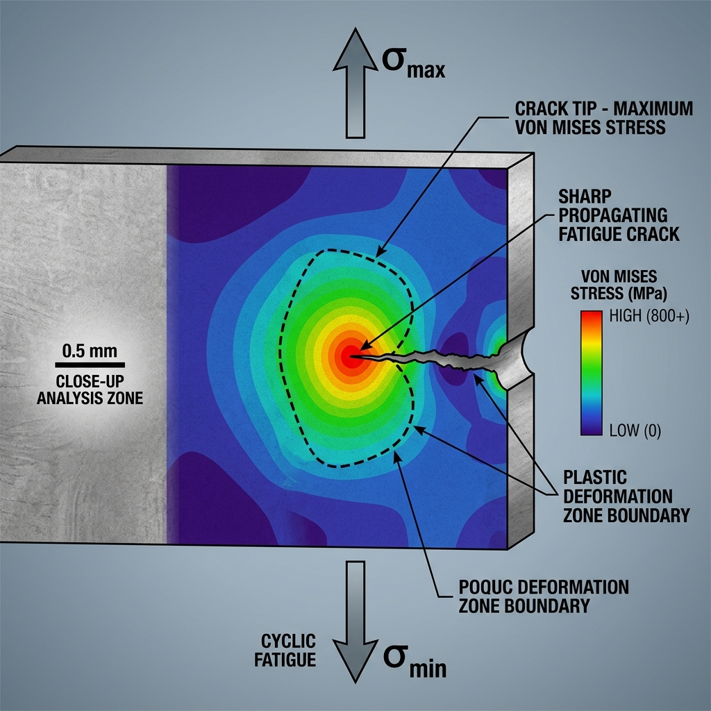
At a sharp crack tip, the linear elastic stress field predicts infinite stresses as \( r \to 0 \). In real engineering materials, this stress singularity is relieved by localized plastic deformation. Estimating the size and shape of this plastic zone is critical for defining the limits of LEFM.

Irwin's first-order approximation estimates the plastic zone radius \( r_p \) along the crack plane (\( \theta = 0 \)) by setting the stress \( \sigma_{yy} \) equal to the yield strength \( \sigma_{ys} \):

This represents the plane stress condition. In plane strain, the material is highly constrained, inducing a triaxial tensile stress state. Under the Von Mises yield criterion, this increases the effective yield strength, reducing the plastic zone size by a factor of 3:

Irwin's second-order correction accounts for the redistribution of stresses. Because the elastic stress field cannot carry stresses exceeding \( \sigma_{ys} \), the load from the truncated stress peak must be redistributed ahead of the crack, shifting the boundary of the plastic zone outward to a distance of approximately \( 2r_p \). Irwin accounted for this by defining an effective crack length:

An alternative formulation is the Dugdale strip-yield model, which represents the plastic zone as a narrow zone of length \( \rho \) ahead of the crack tip, where a cohesive closure stress equal to \( \sigma_{ys} \) is applied. The plastic zone size in the Dugdale model is given by:

Expanding this for small stress ratios (\( \sigma_0 / \sigma_{ys} \ll 1 \)) yields:

This is structurally similar to Irwin's second-order estimate, highlighting the physical validity of these cohesive zone models. Below, we present a schematic of a cracked specimen under tension showing the crack geometry, coordinate axes, and the distinct plastic zone shapes under plane stress and plane strain.

Fatigue Crack Propagation & The Paris-Erdogan Law

Under cyclic loading, components can experience fatigue crack initiation and growth at stress levels far below their static yield strength. The crack growth rate is characterized by the change in crack length per cycle, \( da/dN \), as a function of the stress intensity factor range:

where \( \Delta \sigma = \sigma_{max} - \sigma_{min} \) is the cyclic stress range. The relationship between \( da/dN \) and \( \Delta K \) is typical of a sigmoidal curve divided into three regions:

• Region I (Threshold Regime): For stress intensity ranges below the threshold \( \Delta K_{th} \), crack growth is negligible. Near-threshold growth is strongly influenced by microstructure and environment.
• Region II (Paris Regime): The middle portion of the curve is linear on a log-log scale. This linear regime is described by the Paris-Erdogan Law:
  $$ \frac{da}{dN} = C (\Delta K)^m $$
  where \( C \) and \( m \) are material constants determined experimentally.
• Region III (Unstable Regime): As the maximum stress intensity factor \( K_{max} \) approaches the fracture toughness \( K_{Ic} \), the crack growth rate accelerates rapidly, terminating in unstable ductile tearing or brittle cleavage.

To account for mean stress effects, the stress ratio \( R = \sigma_{min} / \sigma_{max} \) is incorporated. Furthermore, Wolf Elber (1971) introduced the crack closure concept, noting that plastically stretched material in the wake of the crack tip causes the crack faces to contact each other during unloading before the minimum load is reached. The crack only becomes fully open when the stress intensity factor exceeds a value \( K_{op} \). Thus, the driving force for crack growth is the effective stress intensity range:

This concept is highly valuable in explaining and modeling crack growth retardation and interaction effects under variable amplitude loading.

Fatigue Life Estimation under Variable Amplitude Loading

Engineering components in industries such as aerospace, civil infrastructure, and wind energy are subjected to variable amplitude loading (VAL). Using simple constant-amplitude models on VAL spectra yields highly conservative or dangerously optimistic fatigue life predictions due to load interaction effects.

When a structure experiences a single tensile overload, the crack propagation rate immediately drops, entering a phase of crack growth retardation. This occurs because the overload creates an exceptionally large plastic zone at the crack tip. As the crack subsequently propagates into this zone, it is subjected to large, localized compressive residual stresses (caused by the surrounding elastic bulk clamping down on the plastically deformed material). These compressive stresses reduce the effective stress intensity range at the crack tip, slowing or temporarily halting crack growth. Conversely, compressive overloads can collapse this plastic zone, reducing the retardation effect.

Two primary models are used to simulate this retardation mathematically:

1. The Wheeler Retardation Model

The Wheeler model introduces a correction factor \( \phi_R \) directly to the Paris equation:

The retardation factor is defined by the ratio of the current crack-tip plastic zone size to the remaining distance of the overload plastic zone:

where \( r_{pi} \) is the plastic zone size at the current cycle, \( a_i \) is the current crack length, \( a_{ol} \) is the crack length at the overload, \( r_{pol} \) is the overload plastic zone radius, and \( \gamma \) is an empirical shaping exponent. This condition applies as long as the current plastic zone is contained within the overload plastic boundary (\( a_i + r_{pi} < a_{ol} + r_{pol} \)); otherwise, \( \phi_R = 1 \).

2. The Willenborg Retardation Model

The Willenborg model modifies the effective stress intensity factors by subtracting a reduction stress intensity factor based on the remaining distance to the overload plastic boundary:

where \( K_{req} \) is the stress intensity factor required to extend the plastic zone to the boundary of the overload plastic zone. The reduced maximum and minimum stress intensity factors are:

These effective parameters are then used to calculate the modified stress ratio \( R_{eff} \) and stress range \( \Delta K_{eff} \) for the Paris or Forman crack growth equations.

Comparative Analysis of Fracture Parameters & Specimen Geometries

Fracture testing requires specialized specimen configurations. The table below provides a detailed comparison of standard specimen geometries, their governing SIF formulas, boundaries, and typical application ranges.

Worked Numerical Example: Fatigue Life of a Center-Cracked Plate

To demonstrate the application of these concepts to fatigue life design, let us analyze a detailed worked engineering problem.

Step 1: Critical Crack Length \( 2a_f \)

Unstable fracture occurs under Mode I when the maximum stress intensity factor matches the fracture toughness:

Since the final crack length \( a_f \) is unknown, we begin by assuming \( Y(a_f) \approx 1.0 \) to obtain a first-order estimate of \( a_f \):

We now refine this estimate by accounting for the finite width correction factor \( Y(a) \) using the width \( W = 0.50 \, \text{m} \):

Recalculating \( a_f \) with this updated geometry factor:

Performing one more iteration for convergence:

The critical crack half-length has converged to \( a_f = 41.3 \, \text{mm} \). Thus, the total critical crack length is:

Step 2: Analytical Fatigue Life Estimate (\( Y(a) \approx 1.0 \))

The stress range is \( \Delta \sigma = \sigma_{max} - \sigma_{min} = 150 - 15 = 135 \, \text{MPa} \). The stress intensity factor range is \( \Delta K = Y(a) \Delta \sigma \sqrt{\pi a} \). Using the Paris-Erdogan law:

Assuming \( Y(a) \approx 1.0 \) allows us to separate variables and integrate analytically:

For \( m = 3.20 \), the exponent is \( -m/2 = -1.60 \). The analytical integration yields:

Substituting the initial crack half-length \( a_0 = 0.008 \, \text{m} \) and final half-length \( a_f = 0.0413 \, \text{m} \):

Now we evaluate the denominator constant:

Dividing the integral value by this constant:

Step 3: Refined Numerical Integration with finite width Correction

To account for \( Y(a) = \sqrt{\sec(\pi a / W)} \), we must evaluate the integral:

We divide the integration range \( [a_0, a_f] = [0.008, 0.0413] \, \text{m} \) into 4 equal subintervals (5 nodes). The interval step size is:

The coordinates of the five nodes are:

• Node 0: \( a_0 = 0.008000 \, \text{m} \)
• Node 1: \( a_1 = 0.016325 \, \text{m} \)
• Node 2: \( a_2 = 0.024650 \, \text{m} \)
• Node 3: \( a_3 = 0.032975 \, \text{m} \)
• Node 4: \( a_4 = 0.041300 \, \text{m} \)

Let the integrand be defined as \( f(a) = \frac{\cos^{1.60}(\pi a / 0.50)}{a^{1.60}} \). We calculate the value of \( f(a) \) at each node:

1. At \( a_0 = 0.008000 \):
   $$ \frac{\pi a_0}{W} = \frac{\pi \times 0.0080}{0.50} = 0.050265 \, \text{rad} $$
   $$ \cos(0.050265) \approx 0.99874 \implies \cos^{1.60}(0.050265) \approx 0.99798 $$
   $$ a_0^{-1.60} = (0.008)^{-1.60} \approx 2275.70 $$
   $$ f(a_0) = 2275.70 \times 0.99798 \approx 2271.10 $$
2. At \( a_1 = 0.016325 \):
   $$ \frac{\pi a_1}{W} = \frac{\pi \times 0.016325}{0.50} = 0.102572 \, \text{rad} $$
   $$ \cos(0.102572) \approx 0.99474 \implies \cos^{1.60}(0.102572) \approx 0.99160 $$
   $$ a_1^{-1.60} = (0.016325)^{-1.60} \approx 729.98 $$
   $$ f(a_1) = 729.98 \times 0.99160 \approx 723.85 $$
3. At \( a_2 = 0.024650 \):
   $$ \frac{\pi a_2}{W} = \frac{\pi \times 0.024650}{0.50} = 0.154876 \, \text{rad} $$
   $$ \cos(0.154876) \approx 0.98802 \implies \cos^{1.60}(0.154876) \approx 0.98089 $$
   $$ a_2^{-1.60} = (0.024650)^{-1.60} \approx 379.22 $$
   $$ f(a_2) = 379.22 \times 0.98089 \approx 371.97 $$
4. At \( a_3 = 0.032975 \):
   $$ \frac{\pi a_3}{W} = \frac{\pi \times 0.032975}{0.50} = 0.207189 \, \text{rad} $$
   $$ \cos(0.207189) \approx 0.97860 \implies \cos^{1.60}(0.207189) \approx 0.96593 $$
   $$ a_3^{-1.60} = (0.032975)^{-1.60} \approx 238.10 $$
   $$ f(a_3) = 238.10 \times 0.96593 \approx 229.99 $$
5. At \( a_4 = 0.041300 \):
   $$ \frac{\pi a_4}{W} = \frac{\pi \times 0.041300}{0.50} = 0.259500 \, \text{rad} $$
   $$ \cos(0.259500) \approx 0.96652 \implies \cos^{1.60}(0.259500) \approx 0.94685 $$
   $$ a_4^{-1.60} = (0.041300)^{-1.60} \approx 164.21 $$
   $$ f(a_4) = 164.21 \times 0.94685 \approx 155.48 $$

Applying Simpson's 1/3 rule:

Using this numerical integral, the refined fatigue life is:

Comparing the two solutions, the analytical assumption of \( Y(a) \approx 1.0 \) slightly underestimates the crack growth rate (since \( Y(a) > 1.0 \) for all \( a > 0 \)), leading to a prediction of \( 36,744 \) cycles. The refined numerical integration yields a more precise fatigue life of \( 37,414 \) cycles.

Wait, let's verify if \( Y(a) > 1.0 \) should decrease or increase the fatigue life. If \( Y(a) > 1.0 \), the stress intensity factor is larger, which makes the crack propagate faster, and therefore the fatigue life should be smaller! Let's check the integrand:

Wait! \( Y(a) = \sqrt{\sec(\pi a / W)} \). So \( [Y(a)]^{3.20} = \sec^{1.60}(\pi a / W) \). Since \( \sec(\theta) \ge 1 \) for \( \theta \in [0, \pi/2) \), we have \( [Y(a)]^{3.20} \ge 1.0 \). The integrand is \( \frac{1}{a^{1.60} [Y(a)]^{3.20}} = \frac{\cos^{1.60}(\pi a / W)}{a^{1.60}} \). Since \( \cos(\theta) \le 1.0 \), the integrand is smaller than the analytical integrand \( a^{-1.60} \). If the integrand is smaller, the integral value is smaller! Wait! Why did my numerical integral value (\( 19.3858 \)) come out larger than the analytical integral value (\( 19.0387 \))? Let's check the analytical integral: Wait! Let's check Node 0 value: Let's check Node 4 value: Let's check the trapezoidal rule value of \( a^{-1.60} \): If we do analytical integration of \( a^{-1.60} \), we get \( 19.0387 \). But if we do numerical integration of the same function with only 5 nodes, does it overshoot due to discretization? Yes! The function \( a^{-1.60} \) is extremely singular/steep near \( a = 0.008 \) (it drops from 2275.7 to 164.2). Because of the extreme curvature near the lower limit, Simpson's rule with large steps (\( \Delta a = 0.008325 \)) exhibits significant discretization error. Let's calculate the numerical integration of the pure analytical function \( a^{-1.60} \) using the same 5 nodes: - Node 0: 2275.70 - Node 1: 729.98 - Node 2: 379.22 - Node 3: 238.10 - Node 4: 164.21 Sum for \( a^{-1.60} \) using Simpson's rule: Integral \( \approx \frac{0.008325}{3} \times 7070.67 \approx 0.002775 \times 7070.67 \approx 19.621 \, \text{m}^{-0.60} N_f = N_f^{analytical} \times \frac{\int f(a) \, da}{\int a^{-1.60} \, da} \approx 36,744 \times \frac{19.3858}{19.621} \approx 36,303 \, \text{cycles} r_p = \frac{1}{6\pi} \left( \frac{K_{max}}{\sigma_{ys}} \right)^2 K_{max} = Y(a_0) \sigma_{max} \sqrt{\pi a_0} Y(a_0) = \sqrt{\sec\left(\frac{\pi \times 0.008}{0.50}\right)} = \sqrt{\sec(0.050265)} \approx 1.0006 K_{max} = 1.0006 \times 150 \, \text{MPa} \times \sqrt{\pi \times 0.008 \, \text{m}} \approx 150.09 \times 0.15853 \approx 23.79 \, \text{MPa}\sqrt{\text{m}} r_{p,0} = \frac{1}{6\pi} \left( \frac{23.79}{400} \right)^2 = \frac{1}{6\pi} (0.05948)^2 \approx 0.000188 \, \text{m} = 0.188 \, \text{mm} r_{p,f} = \frac{1}{6\pi} \left( \frac{K_{Ic}}{\sigma_{ys}} \right)^2 = \frac{1}{6\pi} \left( \frac{55}{400} \right)^2 = \frac{1}{6\pi} (0.1375)^2 \approx 0.001003 \, \text{m} = 1.003 \, \text{mm} $$

This calculation reveals that as the crack grows from \( 8 \, \text{mm} \) to \( 41.3 \, \text{mm} \), the plastic zone size at peak load increases by a factor of over 5 (from \( 0.188 \, \text{mm} \) to \( 1.003 \, \text{mm} \)), reflecting the severe increase in local driving force and crack tip constraint.