Synthesis and Kinematic Optimization of Compliant Mechanisms in Precision Engineering
Part 1: Physics of Compliance, Pseudo-Rigid-Body Modeling, and Spatial Compliance Matrices
Section 1: Introduction and Physics of Compliance
1.1 The Paradigm Shift in Precision Motion
For centuries, the fundamental tenet of machine design has rested upon the Reuleaux paradigm of rigid-body kinematics. In this classical framework, mechanisms are synthesized by connecting rigid links with kinematic joints (such as revolute, prismatic, or spherical pairs) that constrain relative motion to specific degrees of freedom (DOFs). The structural members are engineered to be as stiff as possible to minimize elastic deformations, which are historically treated as unwanted parasitic disturbances. In precision engineering, however, this rigid-body paradigm encounters fundamental physical limitations. As positioning requirements push down into the sub-micron, nanometer, and sub-nanometer regimes, the microscopic physical phenomena occurring within kinematic joints begin to dominate system behavior.
Compliant mechanisms represent a profound paradigm shift: they achieve motion, force, or displacement transmission through the controlled elastic deformation of flexible members rather than the relative sliding or rolling of rigid components. Instead of suppressing elastic deformation, compliant mechanism design leverages material elasticity as the primary vehicle for motion. This fundamental difference eliminates many of the tribological and mechanical limitations inherent in classical kinematic pairs, making compliance a key enabling technology in semiconductor lithography, scanning probe microscopy, optical alignment systems, micro-electromechanical systems (MEMS), and cryogenic space instrumentation.
1.2 Rigorous Comparison: Rigid-Link vs. Compliant Mechanisms
To systematically understand the engineering trade-offs, we must evaluate both paradigms across key operational parameters. The table below details the performance characteristics of rigid-link mechanisms compared to compliant mechanisms.
1.3 Physical Deficiencies of Rigid Joints in Precision Engineering
To appreciate why compliant structures are indispensable for high-precision positioning, we must mathematically and physically analyze the microscopic deficiencies of traditional kinematic joints.
1.3.1 Backlash and Joint Clearance
For a pin-in-hole revolute joint to exhibit low rotational resistance, there must exist a radial clearance $\Delta r = r_{hole} - r_{pin} > 0$. When the direction of the actuation force reverses, the pin must traverse this clearance envelope before making contact with the opposite side of the hole. This transition zone, where the input motion produces zero output motion, is defined as backlash. Mathematically, if we denote the input displacement as $x_{in}(t)$ and the output displacement as $x_{out}(t)$, the backlash relation can be expressed as:
This clearance introduces a non-linear dead-band zone. In closed-loop feedback control systems, this dead-band introduces a $180^\circ$ phase lag at high frequencies, which triggers limit cycles (hunting) and severely restricts the maximum achievable controller bandwidth. Furthermore, under dynamic conditions, the traversing of the clearance gap leads to micro-impacts, inducing high-frequency structural vibrations and accelerated joint degradation.
1.3.2 Tribological Contact, Friction, and Stick-Slip
Sliding contacts in rigid joints are governed by Coulomb and Dahl friction models. At microscopic scales, surface asperities interlock, requiring a force greater than the dynamic sliding force to initiate motion. This phenomenon, known as static friction ($f_s$), is higher than kinetic friction ($f_k$). The transition from static to kinetic friction leads to the classical "stick-slip" phenomenon, where the system exhibits jerky, discontinuous displacements when low-velocity tracking is attempted.
Furthermore, sliding interfaces are subject to wear according to Archard's Wear Law:
where $V$ is the volume of worn material, $k_w$ is the dimensionless wear coefficient, $F_N$ is the normal load, $d$ is the sliding distance, and $H$ is the material hardness. Over time, wear changes the joint geometry, increases the radial clearance $\Delta r$, and degrades the kinematic accuracy of the mechanism.
1.3.3 Monolithic Fabrication and Assembly Error Stack-up
Traditional mechanisms require the assembly of multiple high-tolerance parts. Each assembly interface introduces geometric errors. If a mechanism has $N$ parts, and the manufacturing tolerance of the $i$-th component in the critical direction is $t_i$, the worst-case assembly tolerance stack-up $T_{worst}$ is:
Even if statistical tolerancing is assumed (assuming independent normal distributions), the root-sum-square tolerance $T_{rss}$ remains a bottleneck:
Compliant mechanisms bypass this limitation by being fabricated monolithically from a single block of material. Techniques such as wire electrical discharge machining (EDM), femtosecond laser micromachining, or photolithography (in MEMS) allow the entire structure (rigid stages and flexible hinges) to be carved out in a single setup. This eliminates assembly errors, minimizes structural interfaces that introduce thermal drift, and guarantees that the geometric relations between axes are defined solely by the precision of the manufacturing tool.
1.3.4 Vacuum and Cryogenic Compatibility
In semiconductor lithography (e.g., Extreme Ultraviolet or EUV systems) and space-borne optical telescopes (e.g., James Webb Space Telescope), mechanisms must operate in high-vacuum ($10^{-6}$ to $10^{-9}$ Torr) or cryogenic (liquid Helium, $4\text{ K}$) environments. Under vacuum conditions, standard hydrocarbons and grease-based lubricants outgas, evaporating and condensing onto nearby optics, which ruins high-value mirrors and lenses. Without lubrication, sliding metallic surfaces in contact experience cold welding (adhesive wear), leading to immediate seizure of the joint. In cryogenic conditions, any remaining lubricant freezes, drastically increasing joint friction. Because compliant mechanisms rely on internal lattice deformation (strain) rather than sliding interfaces, they require no lubrication, produce zero outgassing, and remain fully functional down to Kelvin-scale temperatures.
1.4 Materials Selection Criteria
The engineering challenge of compliant mechanisms lies in their deflection capacity. Because motion is achieved through material deformation, the range of motion is directly constrained by the material's elastic limit. To maximize deflection while maintaining structural integrity, we must establish rigorous material selection metrics.
1.4.1 Derivation of the Yield Strength-to-Modulus Ratio ($\sigma_y/E$)
Consider a simple flat leaf-spring flexure of length $L$, width $w$, and thickness $t$, configured as a cantilever beam. A force $P$ is applied at the free end, causing a transverse deflection $d_y$.
From Euler-Bernoulli linear beam theory, the transverse deflection at the free end is given by:
where $E$ is the Young's modulus of the material, and $I_z = \frac{w t^3}{12}$ is the area moment of inertia of the rectangular cross-section.
The bending moment $M(x)$ along the beam varies linearly, reaching its maximum magnitude at the fixed root ($x = 0$):
The maximum normal bending stress $\sigma_{max}$ occurs at the outer fibers of the cross-section at the fixed root, at a distance $y_c = \pm t/2$ from the neutral axis:
We can express the actuation force $P$ in terms of the target deflection $d_y$ from the deflection equation:
Substituting this expression for $P$ back into the stress equation yields:
To ensure the flexure operates purely within its elastic regime and does not undergo permanent plastic deformation, the maximum stress must not exceed the material's yield strength $\sigma_y$, scaled by a safety factor $S_f$ (where $S_f > 1$):
Substituting the maximum stress relation and solving for the maximum allowable deflection $d_{y,max}$ yields:
This derivation demonstrates that the maximum displacement of a flexure is the product of two distinct terms: a geometric scaling factor $\frac{2 L^2}{3 t S_f}$ and a material performance index $\frac{\sigma_y}{E}$. The ratio $\frac{\sigma_y}{E}$ represents the maximum elastic strain energy density the material can store per unit volume before yielding. Thus, to maximize the deflection range of a compliant mechanism, materials must be selected to maximize this ratio.
1.4.2 Fatigue Behavior under Cyclic Loading
Unlike structural elements in traditional machinery, compliant members are explicitly designed to experience high cyclic bending stresses. Therefore, design static yield strength is insufficient; we must design against high-cycle fatigue (HCF).
Under cyclic loading, micro-cracks nucleate at surface anomalies and propagate through the material. The fatigue life is evaluated using S-N curves, which plot the stress amplitude $S_a$ against the log-scale cycles to failure $N_f$. For materials like steel and titanium, an endurance limit $S_e$ exists, below which the material can theoretically withstand infinite cycles ($N_f > 10^7$). For other materials like aluminum, no true endurance limit exists, and the fatigue strength continues to degrade with cycle count.
When designing flexures, stress concentration effects at fillets and notch transitions must be accounted for using the fatigue notch factor $K_f$:
where $K_t$ is the theoretical geometric stress concentration factor and $q$ is the notch sensitivity of the material. Materials must be selected not only for a high $\sigma_y/E$ ratio but also for low notch sensitivity and high fatigue limits.
1.4.3 Candidate Materials for Compliant Systems
The selection of the optimal material depends on the operating environment and performance requirements. The table below lists primary candidate materials used in compliant mechanisms.
Section 2: Pseudo-Rigid-Body Modeling (PRBM) Formulations
2.1 Large Deflections and the Failure of Linear Beam Theory
The classical Euler-Bernoulli beam equation assumes small deflections, simplifying the curvature expression. The exact curvature $\kappa$ of a planar curve is:
Under the assumption of small slopes ($(\frac{dy}{dx})^2 \ll 1$), the denominator is approximated as $1$, yielding the linear relation $\frac{d\theta}{ds} \approx \frac{d^2y}{dx^2}$. However, in compliant mechanisms, flexible members are specifically designed to undergo large deflections, where the slope $\frac{dy}{dx}$ can exceed $0.5$ (equivalent to angles $> 25^\circ$). In this regime, linear theory introduces severe geometric errors. We must therefore implement the exact elastica equations and solve them using elliptic integrals.
2.2 Exact Mathematical Derivation via Elliptic Integrals
Let us consider a slender cantilever beam of length $L$ and uniform flexural rigidity $EI$. The beam is fixed at the origin ($s=0$, where $s$ is the arc length along the neutral axis) and is subjected to a vertical force $P$ at its free tip ($s=L$).
Let $(x, y)$ be the coordinate of a point along the beam's neutral axis, and let $\theta(s)$ be the slope of the beam at arc length $s$. Let the coordinates of the deflected tip be $(a, b)$, and the slope at the tip be $\theta_0$.
The internal bending moment $M(s)$ at any cross-section located at coordinate $x(s)$ is given by:
According to the Bernoulli-Euler moment-curvature relationship:
To solve this differential equation, we differentiate both sides with respect to the arc length $s$:
Using the kinematic relation $\frac{dx}{ds} = \cos\theta$, we obtain the fundamental governing non-linear ordinary differential equation:
To integrate this equation, we multiply both sides by $\frac{d\theta}{ds}$:
Integrating with respect to $s$ yields:
where $C$ is an integration constant. We evaluate $C$ by applying the boundary condition at the free tip ($s = L$), where the internal bending moment (and thus the curvature) is zero:
Substituting these conditions:
The equation becomes:
Separating variables to solve for the arc length $s$:
Integrating from the fixed base ($s=0, \theta=0$) to the tip ($s=L, \theta=\theta_0$):
To convert this integral into Legendre's standard elliptic form, we introduce the transformation variable $\phi$. Define:
where the modulus $k$ is defined by the boundary condition at the tip where $\theta = \theta_0$ and $\phi = \frac{\pi}{2}$:
Thus:
Differentiating the transformation equation:
Since $\cos\theta = \sqrt{1 - \sin^2\theta}$, and using $\sin\theta = 2 k^2 \sin^2\phi - 1$:
Substituting this into the differential relation:
Now we evaluate the term under the radical in the denominator of the integrand:
Substituting $d\theta$ and $\sqrt{\sin\theta_0 - \sin\theta}$ into the expression for $L$:
The lower limit of integration $\phi_1$ is obtained at $s=0, \theta=0$:
This allows us to express the beam length in terms of Legendre's incomplete elliptic integrals of the first kind, $F(\phi, k)$:
where $K(k)$ is the complete elliptic integral of the first kind.
We can define a dimensionless load parameter $\alpha$:
2.2.1 Exact Coordinates of the Deflected Tip
The horizontal tip coordinate $a$ is derived directly from the moment equation:
At the root $s=0$, $x(0) = 0$ and $\theta(0) = 0$. Substituting these values:
Normalizing by $L$ and substituting $\alpha = \sqrt{\frac{P L^2}{EI}}$:
The vertical tip coordinate $b$ is found by integrating $\frac{dy}{ds} = \sin\theta$ along the beam:
Substituting $\sin\theta = 2 k^2 \sin^2\phi - 1$:
Using the identity $2 k^2 \sin^2\phi - 1 = 1 - 2(1 - k^2 \sin^2\phi)$, we partition the integrand:
This maps directly to incomplete elliptic integrals of the first and second kind ($F$ and $E$, respectively):
Since $\alpha = K(k) - F(\phi_1, k)$, this simplifies to:
Equations for $a/L$ and $b/L$ represent the exact, non-linear coordinates of the deflected cantilever tip. Solving these equations requires numerical evaluation of elliptic integrals, which is computationally expensive for real-time control and synthesis optimization loops.
2.3 The Pseudo-Rigid-Body Model (PRBM) Approximation
To bypass the computational complexity of elliptic integrals, Howell and Midha developed the Pseudo-Rigid-Body Model (PRBM). The PRBM models the complex deflection path of a flexible cantilever beam using a system of two rigid links connected by a pin joint, with a torsional spring at the joint.
Specifically, for a cantilever beam of length $L$: 1. A rigid link of length $\gamma L$ rotates about a virtual pivot located at a distance $(1-\gamma)L$ from the fixed base. 2. The angular deflection of this link is denoted by the pseudo-rigid-body angle $\Theta$. 3. The resistance to deflection is modeled by a torsional spring of stiffness $K_t$ located at the virtual pivot:
where $\gamma$ is the characteristic radius factor, and $K_\Theta$ is the dimensionless stiffness coefficient.
2.3.1 Geometry and Kinematic Matching of $\gamma$
The coordinates of the tip in the PRBM framework are formulated from the kinematics of the rigid-link system:
To determine the optimal value of $\gamma$, we minimize the geometric error between the exact tip coordinates $(a/L, b/L)$ derived from elliptic integrals and the PRBM approximations $(a_{prbm}/L, b_{prbm}/L)$ over a deflection range $0 \le \theta_0 \le \theta_{max}$ (typically $\theta_{max} = 60^\circ$). We formulate the optimization problem:
This optimization yields an optimal characteristic radius factor:
With $\gamma = 0.85$, the maximum error in the predicted tip coordinates is less than $0.5\%$ for deflection angles up to $60^\circ$.
2.3.2 Energy Equivalence and Derivation of $K_\Theta$
The stiffness coefficient $K_\Theta$ is derived by enforcing energy equivalence between the physical beam and the PRBM approximation. The potential strain energy stored in the actual deflecting beam is:
Using the relation $\left(\frac{d\theta}{ds}\right)^2 = \frac{2P}{EI} (\sin\theta_0 - \sin\theta)$, we rewrite the energy integral:
Since the integral of $\sin\theta ds$ is the vertical tip coordinate $b$, we obtain the exact energy relation:
This energy expression matches the physical work done by a constant vertical load $P$ moving through a vertical displacement $b$.
The energy stored in the PRBM torsional spring is:
To equate the two energy models, we must map the physical tip angle $\theta_0$ to the PRBM link angle $\Theta$. Kinematic analysis shows a nearly linear relationship over large deflections:
where $c_\theta$ is a scaling factor. For a vertical force, $c_\theta \approx 1.24$.
Equating $V_{actual}$ and $V_{prbm}$:
Substituting $\alpha^2 = \frac{P L^2}{EI}$ and $\Theta = \frac{\theta_0}{c_\theta}$:
Substituting the exact values of $\alpha$ and $b/L$ calculated from the elliptic integrals for various values of $\theta_0$ into this expression yields $K_\Theta$ as a function of the deflection angle. Minimizing the variation of $K_\Theta$ over the target deflection range ($0$ to $60^\circ$) yields the optimal stiffness coefficient:
Thus, the torque-angle relationship of the virtual spring is defined by:
This formulation allows designers to analyze complex compliant structures using standard rigid-body link-synthesis methods (like the Loop Closure Method) while preserving the non-linear elastica characteristics.
Section 3: Kinematic and Compliance Matrix Formulations
3.1 Screws, Twists, and Wrenches
When deflection amplitudes are small (e.g., within the elastic range of high-performance metals like Titanium or Spring Steel), compliant mechanisms are modeled using the spatial compliance matrix method. This method uses screw theory to model multi-axis flexure hinges.
The infinitesimal displacement of a rigid body is represented by a twist vector $\mathbf{u}$, and the load acting on the body is represented by a wrench vector $\mathbf{F}$. We define these vectors in a local coordinate frame:
where $d_i$ are translation displacements, $\theta_i$ are rotation angles, $f_i$ are forces, and $m_i$ are moments.
The linear relation between the twist and the wrench is governed by the $6 \times 6$ symmetric compliance matrix $\mathbf{C}$:
The inverse of the compliance matrix is the stiffness matrix $\mathbf{K}$:
3.2 Derivation of the Spatial Compliance Matrix for a Rectangular Leaf Flexure
Let us derive the compliance matrix $\mathbf{C}$ for a uniform rectangular leaf flexure of length $L$, width $w$ (along the $y$-axis), and thickness $t$ (along the $z$-axis). The local coordinate system is located at the free end (tip) of the beam, with the $x$-axis directed along the beam's neutral axis towards the fixed root at $x = L$.
We apply Castigliano's Second Theorem to calculate the compliance terms. The theorem states that the displacement $u_i$ corresponding to a load component $F_i$ is the partial derivative of the total strain energy $U$ with respect to that load:
The total strain energy $U$ of a spatial beam including axial tension/compression, bending in two planes, torsion, and shear deformation is:
where:
• $A = w t$ is the cross-sectional area.
• $I_y = \frac{w t^3}{12}$ and $I_z = \frac{w^3 t}{12}$ are the area moments of inertia.
• $J$ is the torsional constant. For a rectangular cross-section ($w \ge t$), $J \approx w t^3 \left[ \frac{16}{3} - 3.36 \frac{t}{w} \left( 1 - \frac{t^4}{12 w^4} \right) \right]$.
• $G = \frac{E}{2(1+\nu)}$ is the shear modulus, and $\nu$ is Poisson's ratio.
• $\alpha_y, \alpha_z$ are the shear correction factors (for rectangular sections, $\alpha_y = \alpha_z = \frac{6(1+\nu)}{5}$).
Let $x$ be the coordinate distance along the beam axis, originating from the free tip ($x=0$) and ending at the fixed base ($x=L$). The internal force and moment resultants at any cross-section $x$ due to the tip wrench $\mathbf{F} = [f_x, f_y, f_z, m_x, m_y, m_z]^T$ are:
Substituting these internal resultants into the strain energy equation:
We derive the compliance coefficients $C_{ij}$ by taking the partial derivatives:
1. Axial compliance ($d_x$ due to $f_x$):
2. Lateral compliance in the $y$-direction ($d_y$ due to $f_y$ and $m_z$):
This yields the direct lateral compliance $C_{22}$ and the cross-coupling compliance $C_{26}$:
3. Vertical compliance in the $z$-direction ($d_z$ due to $f_z$ and $m_y$):
This yields the direct vertical compliance $C_{33}$ and the cross-coupling compliance $C_{35}$:
4. Torsional compliance ($\theta_x$ due to $m_x$):
5. Rotational compliance about the $y$-axis ($\theta_y$ due to $m_y$ and $f_z$):
This yields the direct rotational compliance $C_{55}$ and confirms the symmetric cross-coupling term $C_{53}$:
6. Rotational compliance about the $z$-axis ($\theta_z$ due to $m_z$ and $f_y$):
This yields the direct rotational compliance $C_{66}$ and confirms the symmetric cross-coupling term $C_{62}$:
3.2.2 The Complete $6 \times 6$ Spatial Compliance Matrix
Assembling these terms, the spatial compliance matrix $\mathbf{C}$ of a rectangular leaf flexure at its tip is:
3.3 Coordinate Transformations via the Adjoint Matrix
The compliance matrix derived above is valid only in the local coordinate frame located at the flexure's tip. In a complex compliant mechanism containing multiple flexures, we must transform the individual compliance matrices from their local coordinate frames to a common, global coordinate frame (typically located at the center of gravity or center of stiffness of the moving stage).
Let $A$ be the local coordinate frame at the flexure tip, and $B$ be the target frame. The transformation of a twist $\mathbf{u}_A$ to $\mathbf{u}_B$ is governed by the $6 \times 6$ Adjoint transformation matrix $\mathbf{T}_{Ad}$:
To maintain energy conservation, the work done in both frames must be identical ($W = \mathbf{u}_A^T \mathbf{F}_A = \mathbf{u}_B^T \mathbf{F}_B$). This dictates the transformation of the wrench vector:
Substituting these relations into the local compliance equation $\mathbf{u}_A = \mathbf{C}_A \mathbf{F}_A$:
Thus, the transformed compliance matrix in frame $B$ is:
Let $\mathbf{R}$ be the $3 \times 3$ rotation matrix mapping frame $A$ to frame $B$, and let $\mathbf{r} = [x_d, y_d, z_d]^T$ be the translation vector from the origin of $B$ to the origin of $A$. The Adjoint matrix $\mathbf{T}_{Ad}$ is structured as:
where $\mathbf{S}(\mathbf{r})$ is the skew-symmetric matrix representing the cross-product operation with the translation vector $\mathbf{r}$:
For a translation without rotation ($\mathbf{R} = \mathbf{I}_{3\times3}$), the transformation matrix simplifies to:
3.4 Parallel-Guiding Flexures
A parallel-guiding flexure stage consists of a rigid stage suspended by two identical parallel leaf springs of length $L$, separated by a distance $W$. This design is widely used to achieve linear translation along a single primary axis (e.g., $y$-axis) while constraining all other DOFs.
3.4.1 Boundary Conditions and Stiffness Accumulation
Because the moving stage is rigid and maintains its orientation, the slope at the moving end of both leaf springs is constrained to zero ($\theta_z = 0$). This configuration is a guided-end boundary condition. Let us derive the compliance of a single leaf spring under this constraint.
Using the planar local compliance equations for the bending plane ($xy$):
Imposing the guided constraint $\theta_z = 0$:
Substituting the derived compliance values $C_{62} = C_{26} = -\frac{L^2}{2 E I_z}$ and $C_{66} = \frac{L}{E I_z}$:
This moment must be dynamically generated by the rigid stage to keep the stage's orientation horizontal during translation.
Substituting this expression for $m_z$ back into the lateral displacement equation:
Neglecting the shear deformation term $\frac{\alpha_y L}{G A}$ for slender beams ($L/t \gg 10$), the equivalent lateral compliance of a single guided flexure is:
Because the stage is supported by two identical leaf springs in parallel, the total actuation force $F_{y,total}$ splits equally between them ($F_{y,total} = 2 f_y$). Since both springs experience the same displacement $d_y$, the overall lateral compliance of the parallel-guiding stage is half of the single-spring compliance:
The primary translational stiffness of the stage is:
This stiffness is four times higher than the stiffness of a simple cantilever configuration ($K_{cantilever} = \frac{3EI_z}{L^3}$), showing how boundary constraints modify the stiffness characteristics of compliant mechanisms.
3.4.2 Cross-axis Rotational Stiffness via Separation $W$
The primary function of the parallel-guiding stage is to prevent parasitic rotation of the stage. The rotational stiffness about the $z$-axis ($K_{\theta_z, stage}$) is critical.
To calculate this, we transform the stiffness matrices of both leaf springs to the stage's central coordinate frame. The two springs are located at offsets $y = \pm W/2$ relative to the central frame.
When an external moment $M_z$ is applied to the stage, it rotates by a small angle $\theta_z$. This rotation causes the leaf springs to deform. Specifically, the spring at $+W/2$ is stretched axially, while the spring at $-W/2$ is compressed. The axial displacement of the springs is:
Because the axial stiffness of a single leaf spring is high ($K_{xx} = \frac{E A}{L}$), these axial displacements generate large axial forces:
These forces form a couple that opposes the applied moment:
Adding the intrinsic bending rotational stiffness of the two springs ($2 K_{\theta_z, beam} = \frac{2 E I_z}{L}$), the total rotational stiffness of the stage is:
Since the cross-sectional area $A$ is much larger than the moment of inertia ($I_z = A t^2/12$), the second term dominates:
This relation demonstrates that the rotational constraint stiffness of the stage is proportional to the square of the separation distance $W$. This geometric parameter allows designers to increase rotational stiffness without changing the primary axis translation stiffness $K_{yy, stage}$.
3.5 Parasitic Motion Analysis
A fundamental characteristic of compliant mechanisms is that motion along a primary axis is often coupled with parasitic displacements along other axes. For the parallel-guiding stage, a primary lateral displacement $d_y$ causes a parasitic axial shortening displacement $d_x$.
3.5.1 Mathematical Derivation of the Kinematic Arc-Length Constraint
Because the leaf springs undergo elastic bending, their physical arc length $L$ remains constant (assuming axial tension is small). The relationship between the constant arc length $L$ and the coordinates of the deflected beam is defined by the line integral:
Assuming small-to-moderate deflections ($(\frac{dy}{dx})^2 \ll 1$), we apply a first-order Taylor expansion to the integrand:
Since $d_x$ is small relative to $L$, we can approximate the upper limit of the integral as $L$:
To evaluate this integral, we determine the deflection profile $y(x)$ of the guided beam. For a guided beam under a tip displacement $d_y$, the boundary conditions are:
• At $x=0$: $y(0) = 0$, $\left.\frac{dy}{dx}\right|_{x=0} = 0$
• At $x=L$: $y(L) = d_y$, $\left.\frac{dy}{dx}\right|_{x=L} = 0$
The cubic polynomial that satisfies these four boundary conditions is:
Differentiating this profile with respect to $x$:
Squaring this derivative:
Integrating this expression along the length of the beam:
Using a common denominator of $30$:
Thus:
Substituting this value back into the expression for $d_x$:
This classic equation defines the parasitic axial shortening of a parallel flexure stage. The shortening is non-linear and proportional to the square of the lateral displacement, creating a kinematic coupling effect.
3.5.2 Influence of Axial Forces on Transverse Stiffness
The parasitic axial shortening causes the stage's lateral stiffness to couple with the applied axial force. Let us apply the energy method to evaluate this effect.
Let $F_{axial}$ be an axial force applied to the stage (defined as positive in compression). The total potential energy $V_{total}$ of the system, including the strain energy of the two springs and the potential energy of the axial load, is:
where $K_{yy,0} = \frac{24 E I_z}{L^3}$ is the nominal lateral stiffness without axial load.
Substituting the expression for the parasitic shortening $d_x = 0.6 \frac{d_y^2}{L}$:
The effective lateral stiffness $K_{yy,eff}$ is the second derivative of the potential energy with respect to $d_y$:
This relationship demonstrates that:
1. An axial compressive force ($F_{axial} > 0$) reduces the effective lateral stiffness, making the stage more compliant. If the compressive force reaches $F_{axial} = \frac{20 E I_z}{L^2}$, the lateral stiffness drops to zero, representing structural buckling.
2. An axial tensile force ($F_{axial} < 0$) increases the effective lateral stiffness, making the stage stiffer and more resistant to lateral actuation forces.
This cross-axis coupling introduces challenges in precision control systems, as any variation in axial load (due to assembly misalignments or dynamic forces) directly modulates the lateral transfer function of the actuator.
To isolate stages from parasitic shortening and stiffness modulation, designers implement symmetric folded-beam flexure configurations. In a folded-beam design, the leaf springs are folded back on themselves via an intermediate floating stage. The floating stage moves axially to absorb the parasitic shortening, decoupling the primary stage's lateral translation from axial displacement and load variations.
Compliant Mechanisms Blog Visuals
Figure 1: Dynamic Parallel-Guiding Flexure Stage (Animated)
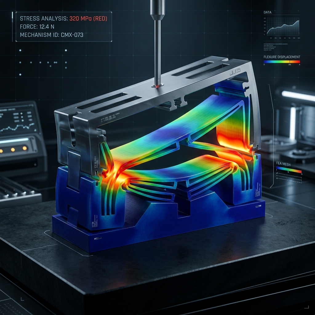
Figure 1: Leaf spring flexures of a parallel-guiding stage bend in an S-shape profile during translation. The stress gradient overlay pulses dynamically: stress is maximum (σmax) at the top and bottom clamps where the bending moment is highest, and zero at the center inflection point.
Figure 2: Pseudo-Rigid-Body Model (PRBM) Comparison (Animated)
Figure 2: The Pseudo-Rigid-Body Model (PRBM) simplifies large-deflection compliant beam analysis by modeling elastomeric bending as a rigid link pivoted at a characteristic joint with a torsional spring. Both profiles are synchronized to deflect identically under load.
Figure 3: FEA Stress-Frequency Resonance Dashboard (Animated)
Figure 3: Simulated mode shape of the compliant flexure stage vibrating at its first natural frequency (f1 = 142.8 Hz). The stress contours pulse at twice the vibration frequency, illustrating how mechanical strain energy alternates between the peak deflection limits, as mapped on the Frequency Response Function (FRF).
Figure 4: Notch-Hinge Flexure Design Blueprint (Static)
Figure 4: Mechanical blueprint details the design parameters of circular and parabolic notch hinges. Linear (X, Y) and angular (θz) degrees of freedom are centered at the notch throat. Circular notch hinges provide cleaner localized rotations, while parabolic profiles distribute stress across wider regions to increase maximum loading capacity.
Section 4: Numerical Worked Example of a Parallel-Guiding Nanopositioning Stage
To bridge the gap between abstract compliant mechanism theory and physical hardware implementation, this section presents a comprehensive, graduate-level numerical design and sizing calculation. We analyze a classic parallel-guiding leaf-spring flexure stage, which is the foundational building block for single-axis nanopositioning systems. By deriving the governing differential equations from first principles and applying boundary conditions, we will determine its primary spring constant, maximum travel range before material yield, parasitic error displacement, and fundamental natural frequency.
4.1 Kinematic and Boundary Condition Configuration
The parallel-guiding stage consists of a rigid moving shuttle (mass $M_s$) suspended relative to a fixed frame by two identical, flat, rectangular leaf springs. We define a Cartesian coordinate system where the $z$-axis lies along the neutral axis of the undeflected leaf springs, the $y$-axis represents the primary direction of motion (transverse deflection), and the $x$-axis lies in the out-of-plane (width) direction. The leaf springs have a free length $L$, width $b$, and thickness $t$.
Each leaf spring is rigidly clamped to the base at $z = 0$ and rigidly clamped to the moving stage shuttle at $z = L$. Because the stage shuttle behaves as a rigid body and is guided by a symmetric pair of flexures, it is constrained against rotation about the $x$, $y$, and $z$ axes. Consequently, as the shuttle translates by a displacement $\delta$ along the $y$-axis, the boundary conditions at the tip ($z = L$) force the slope of the flexure to remain zero. This configuration is mathematically modeled as a guided-clamped beam.
4.2 Mathematical Derivation of Primary Stiffness ($k_y$)
Assuming the leaf springs are slender (slenderness ratio $L/t \gg 20$), we employ the classical Euler-Bernoulli beam theory, which neglects shear deformation and rotatory inertia. For static deflection under a transverse point force $F_1$ and a restoring moment $M_0$ at the guided tip ($z = L$), the transverse deflection curve $w(z)$ is governed by the fourth-order ordinary differential equation:
where $E$ is the Young's modulus of the material and $I$ is the area moment of inertia of the beam cross-section about the bending axis ($x$-axis). For a rectangular cross-section, $I = \frac{b t^3}{12}$. Integrating the governing equation four times with respect to $z$ yields the general polynomial solution:
To solve for the integration constants, we apply the boundary conditions. At the clamped base ($z = 0$), the deflection and slope are zero:
At the guided stage interface ($z = L$), the displacement is equal to the stage travel $\delta$, and the rotation (slope) is constrained to zero:
From the slope boundary condition at $z = L$, we express $C_2$ in terms of $C_1$:
Substituting this relationship into the displacement boundary condition at $z = L$:
Solving for the constants:
Thus, the static elastic deflection curve of the leaf spring is:
The bending moment distribution $M(z)$ along the beam is given by:
The internal shear force $V(z)$ is the derivative of the bending moment:
The transverse force $F_1$ required to deflect a single leaf spring is equal to the magnitude of the shear force at the boundary, $F_1 = -V(L) = \frac{12 EI}{L^3} \delta$. Since the stage incorporates two identical leaf springs working in parallel to guide the shuttle, the total actuation force $F_{total}$ is:
The spring constant (primary stiffness) $k_y$ of the parallel-guiding stage is therefore:
4.3 Stress Analysis and Maximum Displacement ($\delta_{max}$)
The maximum range of travel of a compliant stage is fundamentally constrained by the elastic limit of its material. To avoid permanent set or fatigue failure, the peak stress within the flexures must not exceed the allowable yield strength. The normal bending stress $\sigma(z, y_{fiber})$ at a distance $y_{fiber}$ from the neutral axis (where $y_{fiber} \in [-t/2, t/2]$) is:
The maximum stress magnitude occurs at the outer fibers ($y_{fiber} = \pm t/2$) and at the locations of peak bending moment. Examining the moment distribution $M(z) = \frac{6 EI \delta}{L^2} (1 - 2z/L)$, the maximum moments occur at the boundaries $z = 0$ and $z = L$ with a magnitude of $|M|_{max} = \frac{6 EI \delta}{L^2}$. The peak bending stress in the flexure is:
To prevent yielding, we impose a design criterion based on the material's yield strength $\sigma_y$ and a design factor of safety $S_f$:
Rearranging this inequality for $\delta$ gives the maximum allowable displacement before yielding:
This derivation reveals a critical trade-off: $\delta_{max}$ increases quadratically with flexure length $L$ and decreases linearly with thickness $t$. However, increasing $L$ or decreasing $t$ to achieve larger travel will severely compromise the primary stiffness $k_y$, which scales as $t^3/L^3$. The ratio $\sigma_y/E$ is the material-specific "flex-yield index," showing that materials with high yield strength and low elastic modulus are optimal for maximizing range of motion.
4.4 Kinematic Analysis of Parasitic Displacement ($\Delta z$)
A well-known geometric imperfection of the simple parallel-guiding flexure stage is its kinematic axial retraction. Because the physical arc length of the leaf springs remains constant under moderate deflections (assuming no axial strain or stretching), the horizontal projection of the deflected curve along the $z$-axis must decrease. This results in a parasitic translation of the stage shuttle toward the fixed base.
We compute this retraction $\Delta z$ by parameterizing the deformed neutral axis of a leaf spring by its arc length $s \in [0, L]$. The axial coordinate of the stage shuttle at $s = L$ is:
where $\theta(s)$ is the slope angle of the beam at arc length $s$. Using the Taylor series expansion for the cosine term under the small-slope approximation ($\theta(s) \ll 1$):
Approximating the arc length parameter $s$ with the spatial coordinate $z$ and the slope $\theta$ with the deflection derivative $w'(z)$:
The parasitic displacement $\Delta z$ is the difference between the undeflected length $L$ and the deflected axial position $z_{stage}$:
Differentiating the deflection curve $w(z) = \delta [ 3(z/L)^2 - 2(z/L)^3 ]$ gives:
Squaring this derivative and integrating along the length of the beam:
Substituting this back into the retraction equation yields the classic parasitic retraction formula:
The parasitic axial displacement exhibits a quadratic dependency on the transverse displacement $\delta$. If a nanopositioning stage operates over a large stroke, the axial retraction can become significant, introducing cross-axis coupling error that must be compensated for via multi-axis control or decoupled folded-beam layouts.
4.5 Dynamic Analysis: Equivalent Mass and Fundamental Frequency ($f_n$)
To determine the dynamic performance and bandwidth of the nanopositioner, we model it as a single-degree-of-freedom mass-spring system. The effective stiffness is the primary stiffness $k_y$. The effective dynamic mass $M_{eff}$ must account for both the rigid stage shuttle mass $M_s$ and the distributed mass of the flexing beams. We apply the Rayleigh-Ritz energy method, assuming a harmonic displacement $\delta(t) = \delta_0 \sin(\omega_n t)$.
The total kinetic energy $T(t)$ of the stage is the sum of the kinetic energy of the rigid shuttle and the two leaf springs (each of mass $m_f = \rho b t L$, where $\rho$ is the material density):
The kinetic energy of the rigid shuttle translating at velocity $\dot{\delta}(t)$ is:
For a single leaf spring, the velocity profile $v(z, t)$ of any point along the beam is the time derivative of the deflection shape $w(z, t) = \delta(t) \psi(z)$:
The kinetic energy of one spring is obtained by integrating along the beam length with a linear mass density $\rho A = m_f / L$:
Evaluating the integral:
Thus, the kinetic energy of a single spring is:
Adding the contributions of both springs, the total kinetic energy of the compliant stage is:
Equating this to the kinetic energy of an equivalent lumped single-degree-of-freedom system, $T = \frac{1}{2} M_{eff} \dot{\delta}^2$, we define the effective dynamic mass:
The fundamental natural frequency $f_n$ (in Hz) in the primary actuation direction is:
4.6 Titanium Nanopositioner Sizing Calculations (Ti-6Al-4V Grade 5)
We now perform a step-by-step numerical sizing calculation for a high-performance titanium alloy (Ti-6Al-4V Grade 5) nanopositioning stage. The design parameters and material properties are defined below:
Step 1: Calculate the Area Moment of Inertia ($I$) of a single flexure.
Step 2: Calculate the primary stiffness ($k_y$) of the parallel-guiding stage.
The primary transverse spring constant of the stage is $2736 \text{ N/m}$.
Step 3: Calculate the maximum deflection before yielding ($\delta_{max}$) under design safety factor $S_f = 2.0$.
The stage can travel up to $\pm 6.43 \text{ mm}$ transversely before the outer fiber stress reaches the design limit of $440 \text{ MPa}$ (half the yield strength).
Step 4: Calculate the parasitic displacement ($\Delta z$) at maximum deflection.
At a full transverse displacement of $6.43 \text{ mm}$, the stage shuttle suffers a parasitic axial retraction of $496.6 \ \mu\text{m}$. For a nominal operational displacement of $\delta = 1.0 \text{ mm}$, the parasitic retraction is:
Step 5: Calculate the mass of a single leaf spring ($m_f$).
The mass of each flexure beam is $1.329 \text{ g}$, representing a total suspension mass of $2.658 \text{ g}$.
Step 6: Calculate the effective dynamic mass ($M_{eff}$) of the stage.
Step 7: Calculate the fundamental natural frequency ($f_n$) of the stage.
The fundamental natural frequency of the stage along its primary translation axis is $21.42 \text{ Hz}$.
4.7 Material Selection Trade-offs in Compliant Mechanisms
The choice of flexure material dictates the performance bounds of the compliant mechanism. To benchmark Ti-6Al-4V against other candidate alloys and MEMS-scale materials, the table below compiles key mechanical properties and design indices.
Comparing these properties shows that Titanium Grade 5 offers an exceptional combination of high yield strain (second only to monocrystalline silicon at the micro-scale), moderate density, and low thermal expansion. Aluminum 7075-T6 provides a lightweight alternative, but its high coefficient of thermal expansion ($23.6 \times 10^{-6}/\text{K}$) causes unacceptable thermal drift in nanometer-precision optical and instrumentation platforms. Beryllium Copper (CuBe2) is non-magnetic and highly conductive, making it the choice for compliant electrical contacts despite its high density and high raw material cost. Silicon is superior for micro-machined (MEMS) sensors due to its low thermal expansion, low density, and lack of plastic deformation under moderate loads, though its brittle nature limits its use in macro-scale systems.
4.8 Advanced Effects: Stress-Stiffening and Off-Axis Stiffness Ratios
In precision engineering, we must account for secondary effects that alter the system's stiffness. The primary stiffness equation $k_y(0) = \frac{24 E I}{L^3}$ assumes there is no axial force ($N = 0$) in the leaf springs. However, as the stage undergoes transverse deflection $\delta$, the geometric constraint induces a tensile force $N$ in the springs if the axial boundaries are constrained, or if an external axial force is applied.
To evaluate how an axial tension force $N$ modifies the transverse stiffness of the stage, we write the total potential energy $U$ of a single deformed leaf spring under both bending strain and the work done by the axial force:
Using the cubic deflection profile $w(z) = \delta [ 3(z/L)^2 - 2(z/L)^3 ]$, we compute each integral:
For a stage utilizing two parallel leaf springs, the total potential energy is $U_{total} = 2 U$. The effective transverse stiffness $k_y(N)$ is the second derivative of the potential energy with respect to $\delta$:
This relation demonstrates that:
- Axial tension ($N > 0$) increases the transverse stiffness of the stage, a phenomenon called stress-stiffening.
- Axial compression ($N < 0$) decreases the transverse stiffness, known as stress-softening.
If a compressive load is applied, the transverse stiffness can drop to zero, leading to elastic buckling. The critical buckling load $N_{crit}$ predicted by this energy method is:
The exact Euler buckling load for a guided-clamped beam is $P_{cr} = \frac{\pi^2 EI}{L^2} \approx 9.87 \frac{EI}{L^2}$, demonstrating that our energy method approximation matches the exact solution within $1.3\%$ error.
Finally, we evaluate the off-axis stiffness ratios of the parallel-guiding stage to assess its ability to isolate motion. The stage should be stiff along the axial direction ($z$-axis) and the out-of-plane direction ($x$-axis) to prevent unwanted motion due to off-axis forces. For two parallel leaf springs separated by a distance $d = 40 \text{ mm}$, the stiffnesses are:
- Axial Stiffness ($k_z$): Under tension or compression, the stiffness is governed by the cross-sectional area:
$$ k_z = \frac{2 E b t}{L} = \frac{2 \times (114 \times 10^9 \text{ Pa}) \times 0.012 \text{ m} \times 0.0005 \text{ m}}{0.05 \text{ m}} = 2.736 \times 10^7 \text{ N/m} $$
- Out-of-Plane Stiffness ($k_x$): Bending about the strong axis of the flexure:
$$ k_x = \frac{2 E t b^3}{L^3} = \frac{2 \times (114 \times 10^9 \text{ Pa}) \times 0.0005 \text{ m} \times (0.012 \text{ m})^3}{(0.05 \text{ m})^3} = 1.5746 \times 10^6 \text{ N/m} $$
Comparing these off-axis stiffnesses to the primary transverse stiffness $k_y = 2736 \text{ N/m}$:
The axial stiffness is four orders of magnitude larger than the transverse stiffness, and the out-of-plane stiffness is nearly 600 times larger. This structural anisotropy is the core benefit of compliant guides, providing virtual constraint in all non-actuated degrees of freedom.
Section 6: Topology Optimization and Fabrication of Monolithic Compliant Systems
While simple flexures like leaf springs and circular notch joints can be designed using analytical models, more complex structures—such as multi-degree-of-freedom nanopositioners, displacement amplifiers, and constant-force mechanisms—require advanced design techniques. In these cases, designers use topology optimization to mathematically distribute material within a design domain to achieve the desired compliant behavior.
6.1 The SIMP Method (Solid Isotropic Material with Penalty)
The most common density-based topology optimization method is the Solid Isotropic Material with Penalty (SIMP) technique. The design domain $\Omega$ is discretized into $N$ finite elements. Each element $e$ is assigned a continuous design variable $\rho_e$, representing its relative material density:
where $\rho_{min} = 10^{-3}$ is a small lower bound that prevents the element stiffness matrix from becoming singular. The Young's modulus $E_e$ of each element is interpolated using the power-law relation:
where $E_0$ is the Young's modulus of the solid material, $E_{min}$ is the stiffness of the void phase (typically $E_{min} = 10^{-9} E_0$), and $p$ is the penalization exponent (usually $p = 3$). The role of the exponent $p$ is to penalize intermediate densities (e.g., $\rho_e = 0.5$). Since the stiffness varies non-linearly ($p=3$) while the material volume scales linearly, intermediate densities are structurally inefficient. This drives the optimization toward a binary design of solid ($\rho_e = 1$) or void ($\rho_e = \rho_{min}$).
In classical structural optimization, the objective is to minimize compliance (maximizing stiffness) for a given volume fraction. For compliant mechanisms, however, the goal is to design a structure that is flexible in the actuation direction but stiff enough to withstand reaction forces and off-axis loads.
To achieve this, we optimize the Mutual Strain Energy (MSE), which maximizes the output displacement $d_{out}$ at the output port due to an input force $\mathbf{F}_{in}$ at the input port. To formulate this mathematically, we apply a virtual unit load $\mathbf{L}$ at the output port in the desired direction. The displacement $d_{out}$ is:
where $\mathbf{U}$ is the displacement field produced by the input load $\mathbf{F}_{in}$, satisfying the global equilibrium equation $\mathbf{K}(\boldsymbol{\rho}) \mathbf{U} = \mathbf{F}_{in}$. We define a virtual displacement field $\mathbf{V}$ as the solution to the adjoint equilibrium equation $\mathbf{K}(\boldsymbol{\rho}) \mathbf{V} = \mathbf{L}$. The output displacement can be rewritten as:
The optimization problem is formulated to maximize this displacement while restricting the volume fraction $V^*$ and ensuring the mechanism can resist external loads at the output port (minimizing the output compliance, $\mathbf{U}_{out}^T \mathbf{K} \mathbf{U}_{out}$):
Using the adjoint variable method, the sensitivity of the output displacement with respect to the design variable $\rho_e$ is:
where $\mathbf{k}_0$ is the element stiffness matrix for a fully solid element. To prevent checkerboard patterns (numerical instability characterized by alternating solid and void elements) and mesh dependency, sensitivity or density filters are applied. The density filter updates the element densities using a weighted average of neighbor elements within a filter radius $r_{min}$:
where $N_e$ is the set of elements for which the distance $dist(e, i)$ is less than $r_{min}$, and $H_i = r_{min} - dist(e, i)$ is a linear decay weight function.
6.2 Level-Set Optimization Methods
An alternative to the SIMP method is the level-set method. The level-set method represents the boundaries of the compliant structure explicitly as the zero-contour of a higher-dimensional scalar function $\Phi(\mathbf{x})$. The design domain is divided into solid, boundary, and void regions:
Instead of adjusting element densities, the boundary is deformed by evolving the level-set function $\Phi(\mathbf{x})$ over a pseudo-time parameter $t$ using the Hamilton-Jacobi equation:
where $V_n(\mathbf{x})$ is the normal velocity of the boundary, derived from the shape derivative (sensitivity) of the objective function. The level-set method has several key advantages:
- It eliminates "grey" transition zones of intermediate densities, producing sharp, well-defined boundaries.
- It allows direct integration of geometric constraints, such as minimum member sizes and maximum curvature limits.
- The resulting geometries can be imported directly into CAD software without requiring thresholding or manual cleaning.
6.3 Precision Monolithic Fabrication Techniques
Compliant mechanisms are fabricated as monolithic structures to eliminate joint clearances, assembly tolerances, friction, and hysteresis. However, machining thin flexures within a larger, rigid structure presents unique manufacturing challenges.
Wire Electrical Discharge Machining (Wire EDM):
Wire EDM is the preferred process for manufacturing high-precision metal compliant mechanisms. The process uses a thin brass or copper wire (typically $0.1$ to $0.3 \text{ mm}$ in diameter) acting as an electrode. A series of high-frequency electrical sparks are discharged between the wire and the conductive workpiece in a dielectric bath (deionized water). This erodes the material along a programmed path.
Because there is no physical contact between the tool and the workpiece, wire EDM applies zero mechanical force to the structure. This prevents deflection of thin leaf springs or notch joints during cutting, allowing the fabrication of high-aspect-ratio flexures with dimensional tolerances as tight as $\pm 1 \ \mu\text{m}$.
However, the intense thermal nature of the spark erosion process creates a thin Heat-Affected Zone (HAZ) and a surface recast layer (known as the white layer). This recast layer is brittle, contains tensile residual stresses, and is prone to micro-cracks. Under cyclic loading, these micro-cracks can act as fatigue nucleation sites, reducing the fatigue life of the mechanism. Post-machining treatments, such as chemical etching or electropolishing, are required to remove the recast layer and restore the material's fatigue performance.
Precision CNC Micro-Machining:
CNC micro-milling uses high-speed spindles (40,000 to 100,000 RPM) and small end-mills (down to $100 \ \mu\text{m}$ diameter) to machine complex geometries. Unlike EDM, CNC milling is not restricted to conductive metals and can machine polymers, engineering ceramics, and non-conductive composites.
The primary challenge in micro-milling is tool deflection and workpiece deformation under mechanical cutting forces. As a thin flexure wall is machined, the lateral forces applied by the rotating tool can cause the wall to bend away, resulting in thickness variations or tool breakage.
To mitigate this, designers and machinists use specific toolpaths, such as step-down pocketing, where supporting material is left in place until the final pass. Alternatively, temporary potting compounds (like water-soluble waxes, low-melting-point alloys, or UV-curable polymers) can be poured around the flexure to provide rigid support during machining and then dissolved afterward.
Additive Manufacturing (AM):
Selective Laser Melting (SLM) for metals and Stereolithography (SLA) for polymers enable the fabrication of complex, three-dimensional compliant mechanisms that cannot be produced using traditional subtractive techniques. Additive manufacturing allows the production of multi-axis compliant joints, internal hollow channels, and variable-density lattices.
Despite these capabilities, additively manufactured compliant mechanisms face several limitations:
- Surface Roughness: Metal parts produced via SLM have a high surface roughness ($R_a$ between $5$ and $15 \ \mu\text{m}$) due to partially melted powder particles adhering to the surface. These surface features act as micro-notches, causing stress concentrations that can reduce the fatigue limit by up to $80-90\%$ compared to polished surfaces. Post-processing methods like abrasive flow machining or chemical polishing are critical.
- Microstructural Anisotropy: The layer-by-layer deposition and rapid directional solidification create columnar grains oriented along the build direction. This results in anisotropic mechanical properties, meaning the Young's modulus, yield strength, and fatigue resistance vary depending on the orientation of the flexures relative to the build plate.
- Residual Stresses: The steep thermal gradients during laser melting induce high tensile residual stresses. If not properly managed via stress-relief annealing before removing the part from the build plate, these stresses can cause geometric warping or premature cracking.
6.4 Monolithic Design Constraints and Notch Geometry Optimization
Designing monolithic compliant mechanisms requires careful attention to transition zones where thin flexures connect to thick, rigid blocks. Sharp internal corners act as stress concentrators, multiplying nominal bending stresses and leading to premature failure.
To quantify these stress concentrations, we define the stress concentration factor $K_t$:
For a circular notch hinge with a minimum throat thickness $t_{min}$ and notch radius $R$, the stress concentration factor under bending can be approximated using the empirical relation:
This equation shows that circular notches with small radii $R$ relative to their throat thickness experience high stress concentrations. To reduce peak stress, designers can transition from circular notches to elliptical notches. By increasing the radius along the bending axis, elliptical notches distribute the curvature over a wider region, reducing $K_t$ and increasing the maximum angular deflection.
Advanced designs use Bezier or cubic spline transition curves. Spline curves can be optimized to match the bending moment profile along the flexure, ensuring the stress remains uniform throughout the transition region. This approach can reduce peak stress by up to $30\%$ compared to standard circular fillets.
In addition to stress analysis, physical machining constraints must be integrated into the CAD design:
- Wire EDM Starter Holes: Every closed internal loop in the compliant design requires a pre-drilled starter hole to thread the EDM wire. The design must accommodate these holes without compromising the structural integrity of nearby flexures.
- CNC Tool Radius Clearance: Internal corners machined via CNC milling must have a radius equal to or greater than the radius of the milling tool. Sharp internal corners cannot be directly machined and must be avoided or detailed with relief cuts (often called dog-bone corners).
Section 7: Applications of Compliant Mechanisms in Precision Instrumentation and Aerospace
Compliant mechanisms are used in environments where traditional jointed mechanisms fail due to friction, wear, outgassing, or scaling limitations. This section reviews their application in aerospace, micro-electromechanical systems (MEMS), medical devices, and precision optics.
7.1 Space Exploration and Cryogenic Systems
Space mechanisms must operate in a high vacuum, under extreme thermal cycles (ranging from cryogenic temperatures in shadowed orbits to high temperatures in direct sunlight), and survive launch vibrations. In these conditions, traditional sliding or rolling bearings present significant risks:
- Outgassing: Wet lubricants (greases and oils) evaporate in a vacuum, depositing onto optical surfaces (such as telescope mirrors and sensors) and leaving the joint dry.
- Cold Welding: In the absence of atmospheric oxygen, protective oxide films on metal surfaces are worn away, causing clean metal surfaces in contact to weld together.
- Backlash: Backlash in gears and hinges degrades the positioning accuracy of space antennas and instruments.
Compliant mechanisms eliminate these failure modes. Since they rely on elastic deformation rather than sliding contacts, they require no lubrication, are backlash-free, and do not suffer from cold welding.
Deployable Arrays and Booms:
Tape springs—curved, thin metallic strips similar to tape measures—are widely used as deployable hinges in space applications. When folded, the tape spring stores elastic strain energy. When released, this stored energy deploys the solar array or boom, and the hinge snaps into a rigid state without requiring electric motors, gears, or control electronics.
Cryogenic Mirror Support Flexures:
In space telescopes such as the James Webb Space Telescope (JWST), the primary mirror segments are mounted to a support structure using compliant bipod flexures. The mirrors are made of Beryllium, while the supporting backplane is constructed from Carbon Fiber Reinforced Polymer (CFRP). As the telescope cools to its cryogenic operating temperature of approximately $40 \text{ K}$, the Beryllium mirror and the carbon fiber backplane contract at different rates.
Rigid mounts would transmit these thermal contraction forces directly to the mirror, warping its surface and degrading the telescope's optical performance. To prevent this, the compliant bipod flexures are designed to be extremely soft in the radial direction (absorbing the thermal expansion mismatch) while remaining stiff in the axial and tangential directions to maintain optical alignment and withstand launch loads.
7.2 Micro-Electromechanical Systems (MEMS)
At the micro-scale (micrometers to millimeters), traditional assembly and sliding joints are not viable. As dimensions scale down, the surface-area-to-volume ratio increases, causing surface forces (friction, electrostatic forces, surface tension) to dominate over inertial forces. This makes micro-scale sliding joints highly prone to stiction and wear.
Consequently, MEMS devices rely almost exclusively on compliant mechanisms. Because photolithography and etching processes are monolithic, compliant suspensions can be fabricated directly from the substrate material.
MEMS Sensors:
In MEMS gyroscopes and accelerometers (found in smartphones, vehicles, and guidance systems), a silicon proof mass is suspended by micro-machined compliant silicon springs. When subject to acceleration, the proof mass moves, bending the silicon springs. This deflection is measured capacitively by interdigitated comb structures.
MEMS Actuators:
Electrostatic comb-drive actuators apply voltage to create electrostatic forces, which deflect compliant silicon structures. These actuators are used in micro-mirrors, optical switches, and micro-grippers.
Monocrystalline silicon is an excellent material for compliant MEMS. At room temperature, silicon exhibits perfectly elastic behavior until fracture, with zero dislocation motion. This means the material experiences zero mechanical hysteresis, zero creep, and no fatigue under design stresses, ensuring high repeatability and drift-free operation for micro-sensors.
7.3 Advanced Medical and Surgical Instrumentation
Minimally Invasive Surgery (MIS) and robotic surgical systems require small, precise instruments to operate inside the human body. Traditional micro-instruments use pin joints and cables, which present several operational challenges:
- Sterilization and Cleaning: Blood and biological tissue can become trapped in the small clearances of pin joints, making thorough sterilization difficult.
- Part Loss Risk: The small pins and screws in traditional joints can wear out or loosen, risking component failure inside the patient.
- Backlash: Joint play and friction degrade force feedback (haptics) and compromise positioning accuracy.
Compliant surgical tools address these issues by replacing joints with monolithic flexible structures. These tools can be laser-cut from a single piece of biocompatible material (such as Titanium, PEEK, or Nitinol).
Nitinol (Nickel-Titanium shape memory alloy) is often used in compliant surgical tools due to its superelastic properties. Nitinol can undergo strain levels up to $8\%$ without permanent deformation—ten times higher than spring steel—enabling the design of compact joints that can bend through large angles.
Furthermore, because they are monolithic, these tools have no crevices to trap tissue, simplifying sterilization. The mechanical properties of the compliant joints can also be tailored to act as force-limiters, preventing the tool from applying excessive force to delicate tissues.
7.4 Precision Optical Mounts and Laser Alignment Platforms
Laser systems and precision optics require mirror and lens adjustments with sub-microradian resolution. Traditional kinematic mounts use fine-thread adjustment screws that slide against a metal frame. These interfaces suffer from stick-slip friction, backlash, and long-term drift due to material relaxation or thermal expansion.
Compliant optical mounts solve these issues by replacing sliding contact points with elastic notch hinges. Actuators (such as manual fine-pitch screws or piezoelectric stacks) push against the compliant frame, bending the notch hinges to rotate or translate the optic.
Because the restoring force is purely elastic, compliant optical mounts are backlash-free and exhibit no stick-slip behavior. This allows continuous, repeatable sub-nanometer positioning. Additionally, the mounts can be designed symmetrically to compensate for thermal expansion, maintaining optical alignment over a wide temperature range.