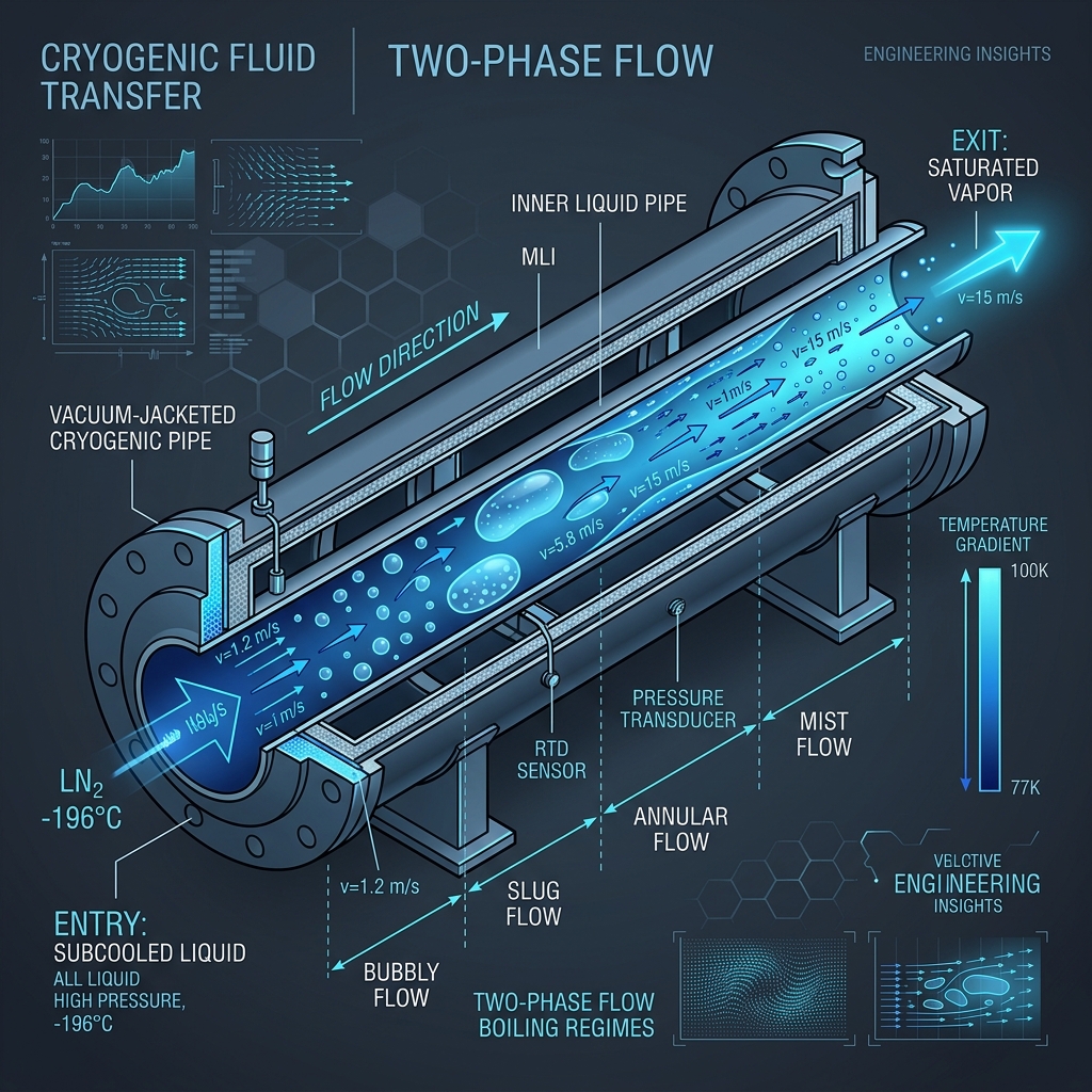
Cryogenic Fluid Transfer & Two-Phase Flow Modeling

Cryogenic fluids, typically defined as liquids with boiling points below 120 K, represent the cornerstone of modern aerospace propulsion, high-energy physics, superconducting applications, and industrial gas distribution. The most common cryogenic liquids—liquid nitrogen (LN2), liquid oxygen (LOX), liquid methane (LCH4), and liquid hydrogen (LH2)—operate at temperatures near absolute zero. Due to their extremely low boiling points, these fluids exist in a state of constant thermal vulnerability. Unlike ambient-temperature liquids like water or hydraulic oil, cryogens have very low latent heats of vaporization and low viscosities. Consequently, even the most advanced vacuum-jacketed piping systems cannot completely eliminate heat leak from the environment. This constant thermal influx drives the fluid into a state of two-phase flow, where liquid and vapor coexist, leading to massive variations in pressure drop, heat transfer rates, flow instability, and cavitation risks.

This technical treatise provides an in-depth engineering analysis of the thermodynamic and hydrodynamic phenomena governing cryogenic fluid transfer. We will explore pool and flow boiling regimes, derive the fundamental equations for void fraction and the Lockhart-Martinelli parameter, analyze cavitation index adjustments due to thermodynamic suppression, evaluate heat transfer correlations, and present a detailed worked numerical example of pressure drop and quality change in a liquid nitrogen transfer line.

1. Thermodynamic and Hydrodynamic Principles of Cryogenic Fluids

Understanding why cryogens behave differently from conventional fluids requires examining their thermodynamic properties. First, their latent heat of vaporization ($h_{fg}$) is remarkably low. For instance, the latent heat of liquid hydrogen is only 446 kJ/kg, compared to 2,260 kJ/kg for water. This means that a minuscule heat leak will vaporize a significantly larger volume of cryogen. Second, the density ratio of liquid to vapor ($\rho_L/\rho_G$) is highly temperature- and pressure-dependent, dropping rapidly as the system approaches the critical point. Third, the dynamic viscosities of both liquid and vapor phases are extremely low, often an order of magnitude lower than water, resulting in high Reynolds numbers and turbulent flow even at modest velocities.

Because cryogenic transfer lines are subjected to continuous heat ingress ($q'$), the fluid experiences forced convection boiling along the flow path. As the fluid absorbs heat, it transitions from a subcooled liquid at the inlet through a series of two-phase flow regimes, eventually reaching saturated vapor or superheated gas if the line is long enough. The spatial distribution of the phases (the flow topology) determines the local pressure gradient and heat transfer coefficient, making the accurate prediction of these flow regimes a vital design requirement.

2. Two-Phase Boiling Regimes

2.1 Pool Boiling Dynamics and the Nukiyama Curve

To understand the physics of boiling, we must first examine pool boiling, which occurs when a heated solid surface is submerged in a stagnant pool of cryogenic liquid. The relationship between the surface heat flux ($q''$) and the excess wall temperature ($\Delta T_e = T_w - T_{sat}$) is represented by the classic Nukiyama boiling curve. In cryogenic systems, the pool boiling curve is compressed toward lower excess temperatures compared to water.

At very low excess temperatures (typically $\Delta T_e < 1\text{ K}$), heat transfer occurs by Natural Convection. The liquid near the wall is heated, rises due to buoyancy, and evaporates at the free pool surface. As $\Delta T_e$ increases, the system enters the Nucleate Boiling regime. Here, microscopic cavities on the rough wall act as nucleation sites where vapor bubbles form. These bubbles grow, detach under buoyancy, and rise, inducing massive localized fluid mixing. This micro-convection effect yields extremely high heat transfer coefficients. The heat flux reaches its peak at the Critical Heat Flux (CHF), which for liquid nitrogen is typically around $100\text{ to }150\text{ kW/m}^2$ at an excess temperature of only $10\text{ to }15\text{ K}$.

Beyond the CHF point, further increases in wall temperature lead to Transition Boiling, where a thin, unstable vapor film begins to form over parts of the surface. Because the thermal conductivity of the vapor is much lower than that of the liquid, the heat flux decreases with increasing wall temperature. When the entire surface becomes blanketed by a stable, continuous vapor layer, the system enters the Film Boiling regime. The minimum temperature required to sustain this stable vapor film is known as the Leidenfrost Point (or the minimum film boiling temperature, $T_{min}$). In cryogenic transfer lines, because the temperature difference between the ambient environment and the cryogen is massive (often exceeding 200 K), the pipe wall is almost always dry, and the system is forced to operate deep within the film boiling regime, despite the low heat flux.

Interactive Dynamics: The Nukiyama Pool Boiling Curve & Boiling Regimes

2.2 Flow Boiling Regimes in Piping Systems

When cryogenic liquid is forced through a horizontal or vertical pipe with wall heat ingress, the boiling process is combined with bulk fluid motion. This forced convection flow boiling results in a series of distinct flow topologies or "regimes" that evolve along the length of the tube:

Single-Phase Liquid Flow: Near the pipe inlet, the fluid remains subcooled or saturated liquid. Heat transfer is governed by forced convection.
Bubbly Flow: As heat leaks through the wall, localized nucleate boiling begins at the inner surface. Small vapor bubbles are swept into the core flow, behaving as a dilute dispersion of gas bubbles in a continuous liquid phase.
Slug Flow: As bubbles grow and coalesce, they form larger, bullet-shaped vapor bubbles (often called Taylor bubbles). These vapor slugs occupy a large fraction of the pipe cross-section and are separated by liquid slugs containing smaller bubbles.
Churn Flow: With higher vapor velocities, the liquid slugs between the Taylor bubbles become unstable and are broken up by the high-speed gas. The flow becomes highly turbulent, oscillatory, and chaotic, with liquid periodically swept upward and falling back.
Annular Flow: At high vapor quality, the gas phase flows at high velocity through the core of the pipe, while the liquid phase is forced to the tube wall, forming a thin, continuous annular film. The shear stress at the gas-liquid interface creates waves, entraining small liquid droplets into the vapor core.
Mist Flow (Post-Dryout): Eventually, the liquid film on the pipe wall evaporates completely (dryout). The wall is contact-free of liquid, and the remaining liquid exists solely as tiny droplets suspended in the continuous vapor core. Heat transfer drops dramatically, and wall temperatures can spike.

3. Governing Equations & Two-Phase Flow Modeling

3.1 Rigorous Derivation of the Void Fraction Equation

The void fraction ($\alpha$) represents the ratio of the volume of the gas phase to the total volume of the flow. In one-dimensional channel flow, this is equivalent to the ratio of the cross-sectional area occupied by vapor ($A_G$) to the total cross-sectional area ($A = A_L + A_G$):

$$ \alpha = \frac{A_G}{A} = \frac{A_G}{A_L + A_G} $$

The vapor quality ($x$) is defined as the ratio of the vapor mass flow rate to the total mass flow rate:

$$ x = \frac{\dot{m}_G}{\dot{m}} = \frac{\dot{m}_G}{\dot{m}_L + \dot{m}_G} $$

Expressing the mass flow rates of the individual phases in terms of their densities ($\rho_G$, $\rho_L$), actual velocities ($u_G$, $u_L$), and cross-sectional areas ($A_G$, $A_L$), we obtain:

$$ \dot{m}_G = \rho_G u_G A_G $$

$$ \dot{m}_L = \rho_L u_L A_L $$

The ratio of the mass flow rate of liquid to that of vapor is:

$$ \frac{\dot{m}_L}{\dot{m}_G} = \frac{1-x}{x} = \frac{\rho_L u_L A_L}{\rho_G u_G A_G} $$

We define the slip ratio ($S$) as the ratio of the actual velocity of the gas phase to that of the liquid phase:

$$ S = \frac{u_G}{u_L} \implies \frac{u_L}{u_G} = \frac{1}{S} $$

We can also express the area ratio in terms of the void fraction. Since $A_G = \alpha A$ and $A_L = (1-\alpha)A$, we have:

$$ \frac{A_L}{A_G} = \frac{(1-\alpha)A}{\alpha A} = \frac{1-\alpha}{\alpha} $$

Substituting the velocity ratio and the area ratio back into the mass flow ratio equation yields:

$$ \frac{1-x}{x} = \left(\frac{\rho_L}{\rho_G}\right) \left(\frac{1}{S}\right) \left(\frac{1-\alpha}{\alpha}\right) $$

To isolate the void fraction, we rearrange the equation:

$$ \frac{1-\alpha}{\alpha} = \left(\frac{1-x}{x}\right) \left(\frac{\rho_G}{\rho_L}\right) S $$

Adding 1 (in the form of $\alpha/\alpha$) to both sides:

$$ \frac{1}{\alpha} = 1 + \left(\frac{1-x}{x}\right) \left(\frac{\rho_G}{\rho_L}\right) S $$

Taking the reciprocal of both sides gives the final expression for the void fraction:

$$ \alpha = \frac{1}{1 + \left(\frac{1-x}{x}\right) \left(\frac{\rho_G}{\rho_L}\right) S} $$

This equation is fundamental in two-phase hydrodynamics. Under the Homogeneous Equilibrium Model (HEM), it is assumed that both phases flow at the exact same velocity, resulting in a slip ratio $S = 1$. In real systems, particularly when the density ratio is high, the vapor phase travels significantly faster than the liquid phase ($S > 1$). A common cryogenic model is Zivi's correlation, which is based on the minimization of kinetic energy:

$$ S_{Zivi} = \left(\frac{\rho_L}{\rho_G}\right)^{1/3} $$

3.2 Rigorous Derivation of the Lockhart-Martinelli Parameter

The Lockhart-Martinelli parameter ($\chi$) is a dimensionless ratio used to determine the frictional pressure drop of a two-phase flow in a pipe by correlating it to single-phase pressure drops. It is defined as:

$$ \chi^2 = \frac{\left(-\frac{dp}{dz}\right)_L}{\left(-\frac{dp}{dz}\right)_G} $$

where $\left(-dp/dz\right)_L$ and $\left(-dp/dz\right)_G$ are the frictional pressure gradients if the liquid phase or gas phase alone were flowing through the entire pipe cross-section at their respective mass flow rates.

Let us derive the expression for turbulent-turbulent flow ($\chi_{tt}$). The frictional pressure gradient for a single-phase fluid flowing in a pipe of diameter $D$ is given by the Fanning equation:

$$ \left(-\frac{dp}{dz}\right) = \frac{2 f \rho u^2}{D} $$

The superficial velocities of the liquid and gas phases are:

$$ u_{s,L} = \frac{G(1-x)}{\rho_L}, \quad u_{s,G} = \frac{G x}{\rho_G} $$

where $G = \dot{m}/A$ is the total mass flux of the mixture. Substituting these velocities into the pressure gradient equation:

$$ \left(-\frac{dp}{dz}\right)_L = \frac{2 f_L G^2 (1-x)^2}{\rho_L D} $$

$$ \left(-\frac{dp}{dz}\right)_G = \frac{2 f_G G^2 x^2}{\rho_G D} $$

For turbulent flow in smooth pipes, the Fanning friction factor can be approximated using the Blasius correlation:

$$ f = C \cdot Re^{-n} $$

The Reynolds numbers for each phase flowing alone are:

$$ Re_L = \frac{G(1-x)D}{\mu_L}, \quad Re_G = \frac{G x D}{\mu_G} $$

Substituting these into the friction factor equations:

$$ f_L = C \left[\frac{G(1-x)D}{\mu_L}\right]^{-n}, \quad f_G = C \left[\frac{G x D}{\mu_G}\right]^{-n} $$

We now plug these back into the individual pressure gradient equations:

$$ \left(-\frac{dp}{dz}\right)_L = \frac{2 C G^{2-n} (1-x)^{2-n} \mu_L^n}{\rho_L D^{1+n}} $$

$$ \left(-\frac{dp}{dz}\right)_G = \frac{2 C G^{2-n} x^{2-n} \mu_G^n}{\rho_G D^{1+n}} $$

Taking the ratio of the two gradients to find $\chi_{tt}^2$:

$$ \chi_{tt}^2 = \frac{\frac{2 C G^{2-n} (1-x)^{2-n} \mu_L^n}{\rho_L D^{1+n}}}{\frac{2 C G^{2-n} x^{2-n} \mu_G^n}{\rho_G D^{1+n}}} = \left(\frac{1-x}{x}\right)^{2-n} \left(\frac{\rho_G}{\rho_L}\right) \left(\frac{\mu_L}{\mu_G}\right)^n $$

For standard turbulent flow in smooth pipes, Blasius gives an exponent of $n = 0.2$. Substituting this value:

$$ \chi_{tt}^2 = \left(\frac{1-x}{x}\right)^{1.8} \left(\frac{\rho_G}{\rho_L}\right) \left(\frac{\mu_L}{\mu_G}\right)^{0.2} $$

Taking the square root of both sides gives the classic Lockhart-Martinelli parameter for turbulent-turbulent flow:

$$ \chi_{tt} = \left(\frac{1-x}{x}\right)^{0.9} \left(\frac{\rho_G}{\rho_L}\right)^{0.5} \left(\frac{\mu_L}{\mu_G}\right)^{0.1} $$

If a different friction factor correlation is used, such as the McAdams correlation where $n = 0.25$, the parameter becomes:

$$ \chi_{tt} = \left(\frac{1-x}{x}\right)^{0.875} \left(\frac{\rho_G}{\rho_L}\right)^{0.5} \left(\frac{\mu_L}{\mu_G}\right)^{0.125} $$

4. Heat Transfer Correlations in Film Boiling

In cryogenic piping systems, the large temperature difference between the ambient environment and the boiling fluid drives the wall heat flux past the Critical Heat Flux (CHF) point. This forces the system into the film boiling regime, where a stable vapor blanket isolates the bulk liquid core from the pipe wall. Heat transfer is highly inefficient, which is desirable to prevent rapid boil-off of liquid, but must be precisely modeled to size vacuum-insulated lines and predict pressure drop.

For film boiling on the outside of horizontal tubes, Bromley's correlation is widely utilized. By analyzing conduction and convection through the vapor film, Bromley derived the following expression for the average heat transfer coefficient ($h_{film}$):

$$ h_{film} = C_{Bromley} \left[ \frac{k_G^3 \rho_G (\rho_L - \rho_G) g h'_{fg}}{\mu_G D \Delta T_e} \right]^{1/4} $$

where $k_G$ is the thermal conductivity of the vapor, $\mu_G$ is its dynamic viscosity, and $h'_{fg}$ is the modified latent heat of vaporization that accounts for the sensible heat required to superheat the vapor film:

$$ h'_{fg} = h_{fg} \left( 1 + 0.4 \frac{c_{p,G} \Delta T_e}{h_{fg}} \right) $$

The theoretical constant $C_{Bromley}$ is $0.62$ for horizontal cylinders. In convective flow boiling inside tubes, Klimenko's correlation is preferred. It categorizes the heat transfer into nucleate and forced-convective regimes, utilizing dimensionless Peclet and Galileo numbers, and has demonstrated superior accuracy in cryogenic systems.

5. Cavitation and Flow Instability in Cryogenic Lines

Cavitation is a significant risk in cryogenic systems, particularly near control valves, pumps, and pipe restrictions. Cavitation occurs when the local static pressure drops below the fluid's saturation vapor pressure, causing vapor bubbles to form. As the fluid moves into a region of higher static pressure, these bubbles collapse violently, creating high-intensity shock waves that erode metal surfaces, generate noise, and restrict flow. The tendency of a system to cavitate is measured by the dimensionless Cavitation Index ($\sigma$):

$$ \sigma = \frac{P - P_v}{\frac{1}{2} \rho_L v^2} $$

where $P$ is the local static pressure, $P_v$ is the vapor pressure at the bulk temperature, and $v$ is the bulk velocity. Cavitation is initiated when $\sigma$ drops below a critical threshold ($\sigma_{crit}$).

In cryogenics, the classic cavitation index is modified by thermodynamic effects. Because cryogenic fluids operate very close to their critical points, the phase change absorbs substantial latent heat from the surrounding liquid, cooling the interface. This local temperature drop lowers the local vapor pressure ($P_v$), which acts to suppress the growth of vapor cavities. This effect, known as the Thermodynamic Suppression Head (TSH), allows cryogenic pumps to operate at a lower Net Positive Suction Head (NPSH) than predicted by standard hydrodynamic models.

Dynamic Cavitation: Bubble Growth, Collapse, & Pressure Profiles in Venturi

Additionally, cryogenic transfer lines are prone to severe flow instabilities. Ledinegg Instability is a static instability that occurs when the system's pressure drop decreases with increasing mass flow rate, creating multiple operating states and leading to flow excursions. Density Wave Oscillations (DWO) are dynamic, self-sustained oscillations caused by delayed propagation of density disturbances along the pipe. The delay in feedback between the vapor generation rate and the inlet flow rate leads to continuous pressure and flow fluctuations, which can damage components and disrupt downstream systems.

6. Comparative Engineering Data

To design effective two-phase transport systems, we must compare the primary thermodynamic and hydrodynamic properties of common cryogenic fluids. The table below lists critical values at their normal boiling points (NBP) at 1 atm:

Cryogen	Normal Boiling Point (K)	Liquid Density (kg/m³)	Vapor Density (kg/m³)	Latent Heat $\text{h}_{\text{fg}}$ (kJ/kg)	Viscosity Ratio $\mu_L/\mu_G$	Critical Temp (K)
Liquid Hydrogen (LH2)	20.3	70.8	1.34	446.0	12.1	33.2
Liquid Nitrogen (LN2)	77.3	808.4	4.61	199.2	27.1	126.2
Liquid Oxygen (LOX)	90.2	1141.0	4.30	213.0	25.6	154.6
Liquid Methane (LCH4)	111.6	422.6	1.82	510.0	22.4	190.6

7. Flow Boiling Regimes Visualization

The schematic diagram below illustrates a pipe section with heat inflow, showing the transition of the cryogenic fluid through various flow boiling regimes (from single-phase liquid on the left to mist flow on the right):

8. Worked Numerical Example

Problem Statement:

A liquid nitrogen (LN2) transfer line is designed to transport subcooled liquid nitrogen at an inlet temperature of 77 K from a pressurized storage dewar to an electronics cooling chamber. The line consists of a smooth horizontal copper tube with an inner diameter of $D = 25\text{ mm}$ ($0.025\text{ m}$) and a total length of $L = 50\text{ m}$.

The system operates under the following conditions:

Inlet mass flow rate: $\dot{m} = 0.15\text{ kg/s}$
Inlet vapor quality: $x_{in} = 0$ (saturated liquid)
Inlet pressure: $P_{in} = 2.0\text{ bar}$ ($0.2\text{ MPa}$)
Uniform heat leak from the environment: $q' = 20\text{ W/m}$

Liquid and vapor properties of Nitrogen at 77 K (saturation) are:

Liquid density: $\rho_L = 808\text{ kg/m}^3$
Vapor density: $\rho_G = 4.6\text{ kg/m}^3$
Latent heat of vaporization: $h_{fg} = 199.2\text{ kJ/kg} = 1.992 \times 10^5\text{ J/kg}$
Liquid dynamic viscosity: $\mu_L = 152 \times 10^{-6}\text{ Pa}\cdot\text{s}$
Vapor dynamic viscosity: $\mu_G = 5.6 \times 10^{-6}\text{ Pa}\cdot\text{s}$

Required Calculations:

Calculate the exit vapor quality ($x_{out}$).
Determine the exit Lockhart-Martinelli parameter ($\chi_{tt}$).
Calculate the exit void fraction ($\alpha_{out}$) using:
- The Homogeneous Equilibrium Model ($S = 1$).
- The Separated Flow Model with Zivi's slip ratio correlation.
Estimate the total pressure drop ($\Delta P_{total}$) across the transfer line using the Homogeneous Equilibrium Model (HEM), accounting for both friction and acceleration.

Step-by-Step Solution:

Step 1: Calculate the exit vapor quality ($x_{out}$)

The total thermal energy leak into the transfer line ($Q_{total}$) is:

          Q_total = q' * L = 20 W/m * 50 m = 1,000 W = 1.0 kW
        

Assuming the liquid enters as a saturated liquid ($x_{in} = 0$), the thermal energy input goes entirely into vaporizing the fluid. The energy balance is:

$$ Q_{total} = \dot{m} \cdot (x_{out} - x_{in}) \cdot h_{fg} $$

Solving for the exit quality ($x_{out}$):

$$ x_{out} = \frac{Q_{total}}{\dot{m} \cdot h_{fg}} = \frac{1000\text{ W}}{0.15\text{ kg/s} \cdot 1.992 \times 10^5\text{ J/kg}} = \frac{1000}{29880} \approx 0.03347 \quad (3.35\%) $$

Step 2: Determine the exit Lockhart-Martinelli parameter ($\chi_{tt}$)

We use the derived formula for the Lockhart-Martinelli parameter for turbulent-turbulent flow:

$$ \chi_{tt} = \left(\frac{1-x_{out}}{x_{out}}\right)^{0.9} \left(\frac{\rho_G}{\rho_L}\right)^{0.5} \left(\frac{\mu_L}{\mu_G}\right)^{0.1} $$

Calculate each term individually:

Quality ratio term: $\left(\frac{1-0.03347}{0.03347}\right)^{0.9} = (28.878)^{0.9} \approx 20.57$
Density ratio term: $\left(\frac{4.6}{808}\right)^{0.5} = (0.005693)^{0.5} \approx 0.07545$
Viscosity ratio term: $\left(\frac{152 \times 10^{-6}}{5.6 \times 10^{-6}}\right)^{0.1} = (27.143)^{0.1} \approx 1.391$

Multiplying these terms together:

$$ \chi_{tt} = 20.57 \cdot 0.07545 \cdot 1.391 \approx 2.159 $$

Step 3: Calculate the exit void fraction ($\alpha_{out}$)

Case A: Homogeneous Equilibrium Model ($S = 1$)

$$ \alpha_{HEM} = \frac{1}{1 + \left(\frac{1-x_{out}}{x_{out}}\right) \left(\frac{\rho_G}{\rho_L}\right)} = \frac{1}{1 + 28.878 \cdot 0.005693} = \frac{1}{1 + 0.1644} \approx 0.8588 \quad (85.88\%) $$

Case B: Separated Flow Model with Zivi Slip

First, calculate the slip ratio using Zivi's relation:

$$ S = \left(\frac{\rho_L}{\rho_G}\right)^{1/3} = \left(\frac{808}{4.6}\right)^{1/3} \approx (175.65)^{1/3} \approx 5.60 $$

Now substitute $S \approx 5.60$ into the void fraction formula:

$$ \alpha_{Zivi} = \frac{1}{1 + \left(\frac{1-x_{out}}{x_{out}}\right) \left(\frac{\rho_G}{\rho_L}\right) S} = \frac{1}{1 + 28.878 \cdot 0.005693 \cdot 5.60} = \frac{1}{1 + 0.9206} \approx 0.5207 \quad (52.07\%) $$

Engineering Note: The homogeneous model drastically overpredicts the void fraction ($85.9\%$ vs. $52.1\%$). In cryogenic applications, vapor travels much faster than liquid due to buoyancy and density differences, making slip models essential for physical accuracy.

Step 4: Estimate pressure drop using the Homogeneous Equilibrium Model (HEM)

The total pressure drop is the sum of the frictional pressure drop and the acceleration pressure drop:

$$ \Delta P_{total} = \Delta P_{fric} + \Delta P_{accel} $$

1. Total Mass Flux ($G$):

$$ G = \frac{\dot{m}}{A} = \frac{\dot{m}}{\frac{\pi}{4} D^2} = \frac{0.15\text{ kg/s}}{\frac{\pi}{4} (0.025\text{ m})^2} \approx 305.58\text{ kg/(m}^2\cdot\text{s)} $$

2. Mixture Density ($\rho_m$) and Viscosity ($\mu_m$):

Under the HEM, properties are calculated as a function of local quality ($x$).

At the inlet ($x = 0$):

          ρ_m,in = ρ_L = 808 kg/m³

          μ_m,in = μ_L = 152 * 10^-6 Pa*s

At the exit ($x = 0.03347$):

$$ \frac{1}{\rho_{m,out}} = \frac{x_{out}}{\rho_G} + \frac{1-x_{out}}{\rho_L} = \frac{0.03347}{4.6} + \frac{0.96653}{808} \approx 0.007276 + 0.001196 = 0.008472\text{ m}^3\text{/kg} $$ $$ \implies \rho_{m,out} \approx 118.0\text{ kg/m}^3 $$

Using McAdams' definition for two-phase dynamic viscosity at the exit:

$$ \frac{1}{\mu_{m,out}} = \frac{x_{out}}{\mu_G} + \frac{1-x_{out}}{\mu_L} = \frac{0.03347}{5.6 \times 10^{-6}} + \frac{0.96653}{152 \times 10^{-6}} \approx 5976.8 + 6358.8 = 12335.6\text{ Pa}^{-1}\cdot\text{s}^{-1} $$ $$ \implies \mu_{m,out} \approx 8.11 \times 10^{-6}\text{ Pa}\cdot\text{s} $$

3. Average Properties for Frictional Pressure Drop:

Since quality $x$ increases linearly with distance $z$ under a uniform heat flux:

$$ x_{avg} = \frac{x_{in} + x_{out}}{2} = 0.01673 $$

The average mixture density corresponding to $x_{avg}$ is:

$$ \frac{1}{\rho_{m,avg}} = \frac{0.01673}{4.6} + \frac{0.98327}{808} \approx 0.003637 + 0.001217 = 0.004854\text{ m}^3\text{/kg} $$ $$ \implies \rho_{m,avg} \approx 206.0\text{ kg/m}^3 $$

The average mixture dynamic viscosity corresponding to $x_{avg}$ is:

$$ \frac{1}{\mu_{m,avg}} = \frac{0.01673}{5.6 \times 10^{-6}} + \frac{0.98327}{152 \times 10^{-6}} \approx 2987.5 + 6468.9 = 9456.4\text{ Pa}^{-1}\cdot\text{s}^{-1} $$ $$ \implies \mu_{m,avg} \approx 1.057 \times 10^{-5}\text{ Pa}\cdot\text{s} $$

4. Average Reynolds Number ($Re_{avg}$) and Friction Factor ($f_{avg}$):

$$ Re_{avg} = \frac{G \cdot D}{\mu_{m,avg}} = \frac{305.58 \cdot 0.025}{1.057 \times 10^{-5}} \approx 722753 \quad (\text{Highly Turbulent}) $$

Using the Blasius correlation for the Darcy friction factor ($f_D = 0.316 \cdot Re^{-0.25}$):

$$ f_{avg} = \frac{0.316}{(722753)^{0.25}} \approx \frac{0.316}{29.15} \approx 0.01084 $$

5. Frictional Pressure Drop ($\Delta P_{fric}$):

$$ \Delta P_{fric} = f_{avg} \cdot \left(\frac{L}{D}\right) \cdot \left(\frac{G^2}{2 \rho_{m,avg}}\right) = 0.01084 \cdot \left(\frac{50}{0.025}\right) \cdot \left(\frac{305.58^2}{2 \cdot 206.0}\right) $$ $$ \Delta P_{fric} = 0.01084 \cdot 2000 \cdot \left(\frac{93379}{412}\right) = 21.68 \cdot 226.65 \approx 4,914\text{ Pa} \approx 4.914\text{ kPa} $$

6. Acceleration Pressure Drop ($\Delta P_{accel}$):

The change in kinetic energy as the liquid evaporates and expands results in an acceleration pressure drop:

$$ \Delta P_{accel} = G^2 \left( \frac{1}{\rho_{m,out}} - \frac{1}{\rho_{m,in}} \right) = 305.58^2 \cdot \left( 0.008472 - \frac{1}{808} \right) $$ $$ \Delta P_{accel} = 93379 \cdot (0.008472 - 0.001238) = 93379 \cdot 0.007234 \approx 675\text{ Pa} \approx 0.675\text{ kPa} $$

7. Total Pressure Drop ($\Delta P_{total}$):

$$ \Delta P_{total} = \Delta P_{fric} + \Delta P_{accel} = 4.914\text{ kPa} + 0.675\text{ kPa} = 5.589\text{ kPa} $$

Discussion of Results:

The total pressure drop is dominated by wall friction ($88\%$ of the total), while the acceleration of the expanding fluid contributes ($12\%$). Because cryogens have highly differing liquid and vapor densities ($\rho_L/\rho_G = 175.65$ for LN2), even small exit quality changes ($3.35\%$) cause the average density to fall from $808\text{ kg/m}^3$ to $206\text{ kg/m}^3$, significantly accelerating the flow and elevating pressure drop. In hydrogen systems, where density ratios are even larger, acceleration pressure drops can exceed frictional pressure drops, leading to potential thermal-acoustic oscillations.

9. Summary and Design Recommendations

Designing cryogenic fluid transfer lines is a delicate balance of mechanical integrity and thermodynamic control. Because of the extremely low latent heat of vaporization of cryogens, heat leak is the primary driver of pressure drops and two-phase transitions. Engineers should employ vacuum-jacketed piping with multi-layer insulation (MLI) to minimize heat leaks below 1-2 W/m. Additionally, to avoid cavitation, liquid transfer lines should be pressurized to maintain sufficient subcooling (cavitation index well above critical). By employing Separated Flow Models and slip ratio corrections like Zivi's, designers can avoid the massive overpredictions of void fractions characteristic of the Homogeneous Equilibrium Model, ensuring reliable performance in aerospace launch facilities and industrial superconducting systems.