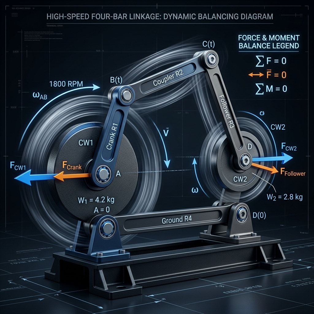
Dynamic Balancing of High-Speed Planar Linkages: Force and Moment Minimization
Graduate-Level Technical Treatise: Kinematics, Force Balancing Theory, and Moment Optimization Foundations
Section 1: Introduction to Linkage Dynamics
1.1 The High-Speed Challenge in Planar Linkages
In the field of high-speed mechanism design, automation, and robotics, the operating frequencies of planar linkages have risen significantly. Planar mechanisms such as four-bar linkages, slider-cranks, and multi-loop configurations are frequently operated at speeds exceeding $15 \text{ Hz}$ to $30 \text{ Hz}$ ($900 \text{ to } 1800 \text{ RPM}$) in pick-and-place packaging, textile weaving, and engine valve gear trains. At these frequencies, the assumption of rigid-body, quasi-static operation is no longer valid. Instead, the design is dominated by the dynamic forces generated by the accelerating masses of the moving links.
Under quasi-static conditions, the forces acting on the joints and linkages are primarily determined by external workloads. However, because inertial forces scale quadratically with the operating speed ($\mathbf{F}_{in} \propto \omega^2$), a tenfold increase in speed yields a hundredfold increase in dynamic forces. These massive, cyclically varying forces and moments are transmitted through the joints and bearings directly to the machine frame and foundation, leading to a host of engineering challenges:
- Structural Vibrations and Foundation Fatigue: The periodic forces transmitted to the machine foundation can excite the natural frequencies of the mounting structure, leading to resonance. This results in high vibration amplitudes, structure-borne noise, and fatigue crack propagation in the mounting frame.
-
Accelerated Joint Bearing Wear: Joint bearings are subjected to severe, fluctuating dynamic loads. According to the classical Lundberg-Palmgren fatigue model, the nominal life of a rolling element bearing, measured in millions of revolutions ($L_{10}$), is given by:
$$ L_{10} = \left( \frac{C}{P} \right)^p $$where $C$ is the basic dynamic load rating, $P$ is the equivalent dynamic load, and the exponent $p$ is $3$ for ball bearings and $10/3$ for roller bearings. Because the dynamic load $P$ is dominated by inertial forces at high speeds ($P \propto \omega^2$), the bearing life scales as:$$ L_{10} \propto \omega^{-2p} $$For a ball bearing ($p=3$), the bearing life is inversely proportional to the sixth power of the speed ($L_{10} \propto \omega^{-6}$). A twofold increase in speed reduces the bearing life by a factor of $64$. Conversely, reducing the transmitted dynamic forces by balancing the mechanism yields a substantial increase in bearing service life.
- Loss of Kinematic Accuracy (Elastodynamics): High-speed linkages cannot be treated as perfectly rigid bodies. The cyclic inertial forces introduce bending moments and axial forces, causing elastic deflections in the links. These deflections lead to path generation errors and positional deviations at the end-effector.
- Acoustic Radiation: High-frequency structural vibrations are transmitted to the surrounding air as acoustic noise. Industrial noise regulations place strict limits on permissible decibel levels to prevent hearing damage and occupational hazards.
- Input Torque Fluctuations: The dynamic acceleration and deceleration of the links require a continuous transfer of kinetic energy to and from the drive motor. This results in large fluctuations in the input torque. The drive motor must be sized to handle these peak torques, leading to larger, less efficient actuators and requiring large flywheels to maintain a constant operating speed.
To address these challenges, mechanical engineers must perform dynamic balancing. Dynamic balancing involves redistributing the mass of the moving links—often through the addition of counterweights or auxiliary links—so that the net force and moment transmitted to the ground are either completely eliminated or minimized.
1.2 Kinematics of the Planar Four-Bar Linkage
A rigorous dynamic analysis requires a complete kinematic model of the linkage. We focus on the planar four-bar linkage, which is the fundamental building block of more complex mechanisms.
Let the linkage consist of four links, numbered sequentially:
- Link 1: The ground frame (fixed).
- Link 2: The input crank, which is connected to the frame at the fixed pivot $O_2$.
- Link 3: The coupler link, which connects joint $A$ (on the crank) to joint $B$ (on the rocker).
- Link 4: The output rocker, which is connected to the frame at the fixed pivot $O_4$.
We define a Cartesian coordinate system with its origin at the fixed pivot $O_2$. The $x$-axis is aligned along the line of centers connecting the two fixed pivots $O_2$ and $O_4$. The fixed pivot $O_4$ is located at the coordinates $(a_1, 0)$, where $a_1$ represents the ground link length. The lengths of the moving links are denoted by $a_2$ (crank $O_2 A$), $a_3$ (coupler $AB$), and $a_4$ (rocker $O_4 B$).
The angular positions of the crank, coupler, and rocker links with respect to the positive $x$-axis are denoted by $\theta_2$, $\theta_3$, and $\theta_4$, respectively. The input crank angle $\theta_2$ is the independent coordinate, while the coupler angle $\theta_3$ and rocker angle $\theta_4$ are the dependent coordinates.
Using complex numbers to represent the link vectors, the loop-closure equation for the mechanism is formulated as:
In complex exponential form, this is written as:
By separating Eq. 1.2 into real and imaginary parts using Euler's identity ($e^{i\theta} = \cos\theta + i\sin\theta$), we obtain:
1.3 Complete Position Analysis
To determine the dependent angles $\theta_3$ and $\theta_4$ for a given crank angle $\theta_2$, we isolate the coupler angle $\theta_3$ in Equations 1.3a and 1.3b:
Squaring both sides of these equations and adding them eliminates the variable $\theta_3$ using the trigonometric identity $\cos^2\theta_3 + \sin^2\theta_3 = 1$:
Expanding Eq. 1.4 yields:
Applying the identities $\cos^2\theta_4 + \sin^2\theta_4 = 1$ and $\cos^2\theta_2 + \sin^2\theta_2 = 1$ simplifies the equation to:
We rewrite Eq. 1.5 in a standard form:
where:
To solve Eq. 1.6, we use the tangent half-angle substitution:
Substituting these into Eq. 1.6 and multiplying by $(1+t_4^2)$ yields:
Rearranging the terms results in a quadratic equation in $t_4$:
The roots of Eq. 1.7 are:
This gives the analytical solution for the rocker angle $\theta_4$:
The two signs ($\pm$) in Eq. 1.9 correspond to the two different assembly modes of the linkage (open and crossed configurations).
We can eliminate $\theta_4$ in a similar manner to solve for the coupler angle $\theta_3$:
where:
Once $\theta_4$ is computed, we can also determine $\theta_3$ directly using the Cartesian components:
1.4 Velocity Analysis
To find the relationship between the angular velocities of the links, we differentiate the complex loop-closure equation (Eq. 1.2) with respect to time:
Using the chain rule, this yields:
where $\omega_j = \dot{\theta}_j$ is the angular velocity of link $j$. Dividing Eq. 1.12 by the imaginary unit $i$ gives:
Separating Eq. 1.13 into real and imaginary parts:
We can express this system of linear equations in matrix form, grouping the dependent angular velocities $\omega_3$ and $\omega_4$ on the left-hand side:
The coefficient matrix on the left-hand side is the kinematic Jacobian matrix $\mathbf{J}$ of the linkage:
The determinant of this matrix is:
Using Cramer's rule, we solve for the coupler angular velocity $\omega_3$:
Similarly, we solve for the rocker angular velocity $\omega_4$:
1.5 Acceleration Analysis
To find the angular accelerations, we differentiate the velocity equation (Eq. 1.12) with respect to time:
Applying the product and chain rules yields:
where $\alpha_j = \dot{\omega}_j$ is the angular acceleration of link $j$. Separating Eq. 1.16 into real and imaginary parts:
Rearranging terms to place the dependent angular accelerations $\alpha_3$ and $\alpha_4$ on the left-hand side:
where:
Solving this system using Cramer's rule yields:
1.6 Mass Center Kinematics
Next, we establish the position, velocity, and acceleration vectors for the centers of mass of the three moving links.
Let $G_k$ be the center of mass of Link $k$ (for $k=2,3,4$). The position of each CoM is defined relative to its respective link axis:
- Link 2 (Crank): The CoM $G_2$ is located at a distance $r_{G2}$ from the pivot $O_2$ at an angular offset $\phi_2$ relative to the link vector $\mathbf{r}_2$.
- Link 3 (Coupler): The CoM $G_3$ is located at a distance $r_{G3}$ from joint $A$ at an angular offset $\phi_3$ relative to the link vector $\mathbf{r}_3$.
- Link 4 (Rocker): The CoM $G_4$ is located at a distance $r_{G4}$ from the pivot $O_4$ at an angular offset $\phi_4$ relative to the link vector $\mathbf{r}_4$.
The position vectors in the complex plane are:
Differentiating these positions with respect to time yields the velocity vectors of the centers of mass:
Differentiating again yields the acceleration vectors:
1.7 Shaking Force and Shaking Moment Definitions
By applying D'Alembert's principle, we define the Shaking Force ($\mathbf{F}_s$) as the net dynamic reaction force transmitted from the moving links to the ground frame. Physically, this is the vector sum of the forces acting on the fixed ground pivots $O_2$ and $O_4$:
where $\mathbf{F}_{21}$ is the force exerted by the crank on the ground, and $\mathbf{F}_{41}$ is the force exerted by the rocker on the ground.
Applying a global force balance to the entire system of moving links shows that the ground reactions must balance the sum of the link inertia forces:
The Shaking Moment ($M_s$) is the net dynamic moment transmitted to the ground frame. Selecting the crank pivot $O_2$ as our reference point, the shaking moment is the sum of the link inertia torques and the moments of the link inertia forces about $O_2$:
Expressing the position and acceleration vectors in Cartesian components ($\mathbf{r}_{Gk} = x_{Gk}\mathbf{\hat{i}} + y_{Gk}\mathbf{\hat{j}}$ and $\mathbf{a}_{Gk} = \ddot{x}_{Gk}\mathbf{\hat{i}} + \ddot{y}_{Gk}\mathbf{\hat{j}}$), the scalar shaking moment about $O_2$ is:
1.8 Dynamic Effects on Mounting Structures
The transmission of these high-frequency shaking forces and moments to the mounting structure can lead to several undesirable dynamic effects. If we model the machine frame and foundation as a single-degree-of-freedom mass-spring-damper system, the force transmissibility ratio $TR$ is given by:
where:
- $r = \omega / \omega_n$ is the frequency ratio, representing the operating frequency divided by the natural frequency of the structure.
- $\zeta$ is the damping ratio of the support structure.
If the frequency ratio $r$ is near $1$, the transmissibility ratio increases significantly, magnifying the transmitted forces. In high-speed systems, the operating frequency often approaches or exceeds the first natural frequency of the mounting frame, leading to resonant excitation. This results in high vibration amplitudes, increased noise levels, and accelerated structural fatigue.
1.9 Detailed Dynamic Joint Force Analysis (Kinetostatics)
To understand the internal load pathways and joint reaction forces, we construct a full kinetostatic model of the moving links. We write the force and moment balance equations for each individual link, treating joint reaction forces as unknowns. Let $\mathbf{F}_{ij} = F_{ijx}\mathbf{\hat{i}} + F_{ijy}\mathbf{\hat{j}}$ be the force exerted by link $i$ on link $j$. By Newton's third law, $\mathbf{F}_{ji} = -\mathbf{F}_{ij}$.
Applying D'Alembert's principle, we set up the equations of motion for each link:
Link 2 (Crank):
where $T_d$ is the driving input torque applied at joint $O_2$.
Link 3 (Coupler):
Link 4 (Rocker):
Equations 1.62, 1.63, and 1.64 form a system of 9 linear algebraic equations in 9 unknowns: the joint forces ($F_{12x}$, $F_{12y}$, $F_{32x}$, $F_{32y}$, $F_{43x}$, $F_{43y}$, $F_{14x}$, $F_{14y}$) and the input drive torque $T_d$. We write this system in matrix form:
where:
The coefficient matrix $\mathbf{A}$ is:
where $x_{GB3} = x_B - x_{G3}$, $y_{GB3} = y_B - y_{G3}$, and the coordinate terms refer to positions relative to the ground. The right-hand side vector $\mathbf{B}$ contains the dynamic inertia terms:
By solving this system at each step of the kinematic cycle, we obtain the profile of all joint reaction forces. The ground reactions $\mathbf{F}_{21} = -\mathbf{F}_{12}$ and $\mathbf{F}_{41} = -\mathbf{F}_{14}$ can then be summed to compute the shaking force, matching the result of Eq. 1.23.
Section 2: Shaking Force Balancing Theory
2.1 The Stationary Center of Mass Condition
For the shaking force $\mathbf{F}_s$ to be identically zero at all times, the total center of mass of the mechanism must remain stationary. The total mass of the moving parts of the linkage is:
The position vector representing the center of mass of the entire linkage, $\mathbf{r}_S$, is:
Substituting this definition into the shaking force expression:
If the mass distribution is designed such that the total center of mass is stationary, then:
To achieve this condition, the mass-center vector $\mathbf{r}_S$ must be independent of the time-varying joint angles $\theta_2$, $\theta_3$, and $\theta_4$. We solve this mathematical problem using the method of linearly independent vectors.
2.2 Method of Linearly Independent Vectors
Developed by Berkof and Lowen (1969), the method of linearly independent vectors provides a systematic algebraic technique to balance linkages. The method proceeds by expressing the total mass-center vector $\mathbf{M} \mathbf{r}_S$ as a linear combination of the time-varying unit vectors that describe the angular orientation of each link.
We write the total mass-center vector in terms of the complex coordinates of the centers of mass:
Substituting the CoM position equations (Eq. 1.20a-c):
Grouping the coefficients of the time-varying unit vectors $e^{i\theta_2}$, $e^{i\theta_3}$, and $e^{i\theta_4}$:
Equation 2.2 represents the mass-center vector in terms of three time-varying unit vectors. However, because of the closed-loop nature of the four-bar linkage, these three vectors are not linearly independent. They are constrained by the loop-closure equation (Eq. 1.2):
We can eliminate one of the time-varying vectors from the mass-center expression. Typically, we eliminate the coupler term $e^{i\theta_3}$ because adding heavy counterweights to the coupler (which undergoes complex general planar motion) significantly increases the shaking moment and input torque.
Expressing the unit vector $e^{i\theta_3}$ from the loop-closure equation:
Substituting Eq. 2.3 into Eq. 2.2:
Now, we collect terms to separate the constant term and the coefficients of the remaining time-varying unit vectors, $e^{i\theta_2}$ and $e^{i\theta_4}$:
In Eq. 2.4, the unit vectors $e^{i\theta_2}$ and $e^{i\theta_4}$ are linearly independent for a general four-bar linkage because the angles $\theta_2$ and $\theta_4$ cannot maintain a constant relation across the full cycle of motion. Therefore, for the total center of mass vector $\mathbf{r}_S$ to remain constant throughout the cycle, the coefficients of the time-varying vectors $e^{i\theta_2}$ and $e^{i\theta_4}$ must be identically zero:
If Equations 2.5 and 2.6 are satisfied, the total mass-center vector simplifies to:
Because the position of the total center of mass is stationary, the net shaking force is completely eliminated.
2.3 Derivation of Counterweight Parameters
To satisfy the balancing conditions in Equations 2.5 and 2.6, we must adjust the mass distributions of Link 2 and Link 4. In general, the mass properties of the original coupler link (Link 3) are fixed by operational requirements. Therefore, we introduce counterweights on Link 2 (crank) and Link 4 (rocker).
Let the original mass properties (before balancing) of the crank and rocker be:
- Crank (Link 2): Original mass $m_{20}$, CoM distance $r_{G20}$, and phase angle $\phi_{20}$.
- Rocker (Link 4): Original mass $m_{40}$, CoM distance $r_{G40}$, and phase angle $\phi_{40}$.
We add a counterweight of mass $m_{cw2}$ at a radial distance $r_{cw2}$ and angular position $\theta_{cw2}$ on Link 2. The combined mass properties of Link 2 are:
Similarly, we add a counterweight of mass $m_{cw4}$ at a radial distance $r_{cw4}$ and angular position $\theta_{cw4}$ on Link 4. The combined mass properties of Link 4 are:
Substituting the expressions for the combined links (Eq. 2.8b and Eq. 2.9b) into the force balancing conditions (Eq. 2.5 and Eq. 2.6):
Isolating the counterweight parameters on the left-hand side yields two vector equations in the complex plane:
To find the physical parameters (mass-radius product and phase angle), we resolve Eq. 2.10 and Eq. 2.11 into their real and imaginary components.
For the crank counterweight (Link 2), let:
The mass-radius product of the crank counterweight is:
And the phase angle $\theta_{cw2}$ is:
For the rocker counterweight (Link 4), let:
The mass-radius product of the rocker counterweight is:
And the phase angle $\theta_{cw4}$ is:
Once the designer selects a physically feasible radius ($r_{cw2}$ and $r_{cw4}$), the required counterweight masses ($m_{cw2}$ and $m_{cw4}$) are computed directly from the mass-radius products.
By implementing these counterweight parameters, the net dynamic shaking force transmitted to the frame is theoretically reduced to zero. However, this force balance is achieved at the expense of adding substantial mass to the moving links, which increases the shaking moment and the torque required to drive the linkage.
2.4 Lumped Mass Approximation: Physical Insight into Force Balancing
The method of linearly independent vectors can be understood physically using a lumped mass approximation. In this approach, we replace the distributed mass of the coupler (Link 3) with a statically equivalent system of three concentrated point masses: $m_{3A}$ located at joint $A$, $m_{3B}$ located at joint $B$, and a remaining mass $m_{3G}$ at the coupler's center of mass $G_3$.
To ensure the lumped system is statically equivalent to the original coupler, the concentrated masses must satisfy the following conditions:
where $\mathbf{r}_{A/G3}$ and $\mathbf{r}_{B/G3}$ are the position vectors of joints $A$ and $B$ relative to the center of mass $G_3$.
If we model the coupler by lumping its mass only at the two joint endpoints $A$ and $B$, we set $m_{3G} = 0$. The resulting two-mass model is statically equivalent if:
where $l_{3A}$ is the distance from $A$ to $G_3$, and $l_{3B}$ is the distance from $B$ to $G_3$.
By replacing the coupler with these two lumped masses, we apportion the coupler's mass between the crank tip $A$ and the rocker tip $B$. The mass concentrated at joint $A$ ($m_{3A}$) rotates in a circle of radius $a_2$ and can be balanced by a counterweight on the crank (Link 2). The mass concentrated at joint $B$ ($m_{3B}$) oscillates with the rocker and can be balanced by a counterweight on the rocker (Link 4).
However, this two-mass model is not dynamically equivalent because it does not preserve the coupler's mass moment of inertia:
The difference $\Delta I_3 = I_{G3} - I_{G3}^*$ is the inertia error. This error generates an unbalanced dynamic moment during operation, contributing to the shaking moment and causing input torque fluctuations. This highlights the trade-off in linkage balancing: complete force balancing can be achieved using static lumping, but the dynamic mismatch (inertia error) remains, generating an unbalanced shaking moment.
Section 3: Shaking Moment Minimization
3.1 Analytical Derivation of the Shaking Moment
We now derive the shaking moment equation for a four-bar linkage about the crank pivot $O_2$. As defined in Eq. 1.24, the shaking moment $M_s$ consists of the inertia torques and the moments of the inertia forces:
Let us evaluate the cross-product term $\mathbf{M}_{Gk} = \mathbf{r}_{Gk} \times (m_k \mathbf{a}_{Gk})$ for each link individually.
3.1.1 Crank Moment Contribution (Link 2)
The position and linear acceleration of the crank's center of mass $G_2$ are:
Taking the cross product of these two complex numbers:
Using the cross-product properties of complex vectors in the plane:
This simplifies the expression to:
Adding the direct inertia torque contribution, the total shaking moment contribution from Link 2 is:
where $I_{O2}$ is the mass moment of inertia of Link 2 about the fixed pivot $O_2$.
3.1.2 Rocker Moment Contribution (Link 4)
The position and linear acceleration of the rocker's center of mass $G_4$ are:
Computing the cross product:
Expanding the terms:
The unit vector $\mathbf{\hat{i}}$ corresponds to $e^{i0}$. The planar cross products are:
Substituting these expressions back into the equation:
Adding the direct inertia torque contribution, the total shaking moment contribution from Link 4 is:
where $I_{O4} = I_{G4} + m_4 r_{G4}^2$ is the mass moment of inertia of Link 4 about the fixed pivot $O_4$.
3.1.3 Coupler Moment Contribution (Link 3)
The position and linear acceleration of the coupler's center of mass $G_3$ are:
Computing the cross product:
Expanding this cross product yields four terms:
-
$$ T_1 = a_2^2 \left( e^{i\theta_2} \times \left( i \alpha_2 - \omega_2^2 \right) e^{i\theta_2} \right) = a_2^2 \alpha_2 \mathbf{\hat{k}} $$
-
$$ T_2 = r_{G3}^2 \left( e^{i(\theta_3 + \phi_3)} \times \left( i \alpha_3 - \omega_3^2 \right) e^{i(\theta_3 + \phi_3)} \right) = r_{G3}^2 \alpha_3 \mathbf{\hat{k}} $$
-
$$ T_3 = a_2 r_{G3} \left[ e^{i\theta_2} \times \left( i \alpha_3 - \omega_3^2 \right) e^{i(\theta_3 + \phi_3)} \right] = a_2 r_{G3} \left( \alpha_3 \cos(\theta_3 + \phi_3 - \theta_2) - \omega_3^2 \sin(\theta_3 + \phi_3 - \theta_2) \right) \mathbf{\hat{k}} $$
-
$$ T_4 = a_2 r_{G3} \left[ e^{i(\theta_3 + \phi_3)} \times \left( i \alpha_2 - \omega_2^2 \right) e^{i\theta_2} \right] = a_2 r_{G3} \left( \alpha_2 \cos(\theta_3 + \phi_3 - \theta_2) + \omega_2^2 \sin(\theta_3 + \phi_3 - \theta_2) \right) \mathbf{\hat{k}} $$
Summing these four terms:
Adding the direct inertia torque contribution, the total shaking moment contribution from Link 3 is:
where $I_{O3} = I_{G3} + m_3 r_{G3}^2$ is the moment of inertia of Link 3 about joint $A$.
3.1.4 Total Shaking Moment Equation
The total shaking moment $M_s$ about the crank pivot $O_2$ is the sum of the individual link contributions:
Substituting Eq. 3.3, 3.5, and 3.7:
Equation 3.8 represents the general shaking moment about $O_2$ for any planar four-bar linkage.
If the linkage is already force-balanced by counterweights on the crank and rocker, the force balancing conditions (Eq. 2.5 and Eq. 2.6) must hold. Let us examine how these conditions simplify the shaking moment.
From the rocker force balancing condition (Eq. 2.6):
Equating the real and imaginary parts:
Let us substitute these relations into the rocker component of the shaking moment:
Expanding the trigonometric terms:
Thus:
Substituting these back, the rocker moment contribution reduces to:
Using Eq. 3.9, we express the shaking moment of a force-balanced four-bar linkage in a simplified form that is independent of the rocker's center of mass position $r_{G4}$:
where $I_{O2}^*$, $I_{O3}^*$, and $I_{O4}^*$ are the moments of inertia of the force-balanced links, which now include the contributions of the added counterweights.
3.2 Proof of the Impossibility of Complete Passive Moment Balancing
A fundamental question in linkage design is: Can we design a set of passive counterweights to eliminate the shaking moment $M_s$ completely, just as we did for the shaking force $\mathbf{F}_s$?
To answer this, we apply the method of linearly independent vectors to the shaking moment expression and attempt to set the coefficients of all time-varying terms to zero.
We assume the input crank rotates at a constant angular velocity, so $\omega_2 = \text{constant}$ and $\alpha_2 = 0$. Under this condition, the shaking moment equation (Eq. 3.8) simplifies to:
Observe that Eq. 3.11 contains the dependent angular velocities squared ($\omega_3^2$, $\omega_4^2$) and the dependent angular accelerations ($\alpha_3$, $\alpha_4$). From our kinematic derivations (Eq. 1.60, 1.61, 1.18, and 1.19), these variables are highly non-linear functions of the input angle $\theta_2$.
Because the linkage undergoes cyclic motion, any kinematic variable $f(\theta_2)$ can be represented by a Fourier series in terms of the crank angle $\theta_2$:
The Fourier coefficients in Eq. 3.12 are calculated using the Euler-Fourier integrals:
For the shaking moment to be identically zero for all crank positions, every single Fourier coefficient must vanish:
This represents an infinite set of algebraic constraints. However, the designer has only a finite number of physical design variables to adjust. Even if we allow counterweights on all three moving links, we have only six design variables: the mass-radius products and phase angles of the three counterweights ($m_{cw2}r_{cw2}, \theta_{cw2}, m_{cw3}r_{cw3}, \theta_{cw3}, m_{cw4}r_{cw4}, \theta_{cw4}$).
Mathematically, we cannot satisfy an infinite number of independent Fourier coefficient constraints with a finite number of design variables.
To illustrate this impossibility from a physical perspective, let us analyze the rotational inertia forces. The angular accelerations of the coupler and rocker, $\alpha_3$ and $\alpha_4$, are driven by the changing geometry of the linkage. The inertial torques $I_{O3}\alpha_3$ and $I_{O4}\alpha_4$ vary in a complex, non-harmonic manner.
A passive counterweight attached to a rotating link can only generate inertial forces that are directed radially (centripetal forces) or tangentially (tangential acceleration forces). For Link 2 and Link 4, which pivot about fixed points, their counterweights can only apply moments about $O_2$ and $O_4$ that are proportional to their own angular accelerations and the squares of their own angular velocities. These counterweights cannot generate the non-harmonic, high-frequency force components required to cancel the inertial forces of the coupler (Link 3), which undergoes complex translation and rotation.
If we attempt to set up the method of linearly independent vectors for the shaking moment, we find that the time-varying coefficients cannot be grouped into a set of independent vectors whose coefficients can be set to zero. For example, to eliminate the term containing $\alpha_3$, we would require the moment of inertia of the coupler to be zero ($I_{O3} = 0$), or even negative, which is physically impossible for any real mass distribution.
Thus, we establish the fundamental theorem of linkage balancing:
"It is physically impossible to achieve complete shaking moment balancing in a planar four-bar linkage using passive counterweights alone, without adding auxiliary links or active elements."
3.3 Optimization Criteria for Shaking Moment Reduction
Because complete shaking moment balancing is impossible with passive counterweights, we must treat the design of the counterweights as a optimization problem. The goal is to find the mass distributions of the links that minimize the shaking moment over a full cycle of operation, subject to physical constraints.
Let the vector of design variables be:
3.3.1 Objective Functions
Depending on the application, different mathematical metrics are used to define the "minimization" of the shaking moment:
1. Root-Mean-Square (RMS) Shaking Moment: This metric minimizes the total vibrational energy transmitted over a cycle. It is the most common objective function for vibration and noise reduction:
where $T = 2\pi/\omega_2$ is the period of one operating cycle.
2. Peak-to-Peak Shaking Moment: This metric minimizes the maximum shock or structural load experienced by the foundation:
3.3.2 Multi-Objective Formulations and the Force-Moment Trade-Off
If we enforce complete shaking force balancing (using Equations 2.8 to 2.13), the counterweights add significant mass to the crank and rocker. This increases their moments of inertia ($I_{O2}$ and $I_{O4}$), which directly increases the shaking moment.
To resolve this conflict, we allow partial force balancing. We relax the requirement that the shaking force must be exactly zero, and search for a compromise that reduces both the shaking force and the shaking moment. This is formulated as a weighted multi-objective optimization problem:
where:
- $w_f$, $w_m$, and $w_t$ are weighting factors that represent the designer's priorities.
- $F_{ref}$, $M_{ref}$, and $T_{ref}$ are normalizing scale factors, typically chosen as the peak values of the unbalanced linkage.
- $T_d(t, \mathbf{x})$ is the dynamic driving torque required to maintain constant input speed, and $T_{d, avg}$ is its cycle average.
By varying the weights ($w_f, w_m$), we can map out a Pareto frontier that shows the optimal trade-off between shaking force and shaking moment, as illustrated conceptually in the table below:
3.3.3 Geometric and Physical Constraints
The optimization process must satisfy several geometric and physical constraints to ensure the resulting linkage is manufacturable:
- Space Envelope Constraints: The counterweights must not collide with other moving links, fixed joints, or the surrounding machine housing. This restricts the maximum radial distance $r_{cw}$ and the thickness of the weights.
- Mass Budgets: Adding too much mass can overload the main bearings and increase the required starting torque, which can trip the motor drives.
- Link Strength and Stiffness: The centrifugal forces generated by the counterweights introduce large bending moments on the link shafts, requiring thicker structures that must be checked against mechanical stress limits.
In practice, these optimization problems are solved using numerical algorithms such as Sequential Quadratic Programming (SQP) or genetic algorithms. In Part 2 of this post, we will implement these algorithms in MATLAB and Python, demonstrating how to compute the optimal counterweight parameters for a high-speed pick-and-place robot linkage.
3.4 Advanced Mechanical Balancing Techniques
Because passive counterweights cannot completely eliminate the shaking moment, advanced dynamic balancing techniques have been developed. These methods either cancel the shaking moment using auxiliary mechanisms or introduce active components:
-
Duplicated Symmetric Mechanisms: One of the most effective ways to balance both shaking force and shaking moment is to use two identical linkages mounted in mirror-image configuration. The two mechanisms are driven in opposition, meaning that when one crank rotates clockwise, the other rotates counterclockwise at the same speed.
Let $\mathbf{F}_{s1}$ and $M_{s1}$ be the shaking force and moment of the first linkage, and $\mathbf{F}_{s2}$ and $M_{s2}$ be those of the second linkage. Because of the symmetry:$$ \mathbf{F}_{s2}(t) = -\mathbf{F}_{s1}(t) \quad \text{and} \quad M_{s2}(t) = -M_{s1}(t) \quad \text{(Eq. 3.70)} $$Summing the forces and moments transmitted to the frame:$$ \mathbf{F}_{s, total} = \mathbf{F}_{s1} + \mathbf{F}_{s2} = \mathbf{0} \quad \text{and} \quad M_{s, total} = M_{s1} + M_{s2} = 0 \quad \text{(Eq. 3.71)} $$This yields complete force and moment balancing across the entire cycle of motion. This approach is widely used in high-end industrial pick-and-place systems and high-speed sorting machines, though it doubles the number of parts, increasing the cost, size, and cost of the machine. - Gear-Driven Counter-Rotational Shafts (Lanchester Balancer): In internal combustion engines and slider-crank linkages, gear-driven shafts are used to balance the second harmonic ($n=2$) of the shaking force or moment. A pair of counter-rotating shafts with eccentric weights are geared to run at twice the input crank speed. The centrifugal forces generated by these weights cancel the second harmonic of the inertial forces.
- Auxiliary Balancing Links: An auxiliary dyad (a two-link combination) can be added to the mechanism to balance the shaking moment. The dyad is designed to move out-of-phase with the primary linkage, so that its inertial torque cancels the shaking moment of the main mechanism.
- Active Moment Balancers: Active moment balancers use a servomotor to drive a rotating mass in a non-harmonic, pre-programmed speed profile. The motor speed is controlled in real-time to match and cancel the shaking moment of the primary linkage. While highly effective, active balancers require high-bandwidth control systems and consume additional electrical energy.
These advanced techniques provide valuable solutions for applications where passive optimization is insufficient to meet strict vibration and noise limits.
Linkage Balancing Visualizations
An interactive suite of visualizations showing the kinematics, shaking forces, polar shaking moments, and vector loop equations of a Grashof crank-rocker mechanism in unbalanced and balanced configurations.
Figure 1: Kinematics of the Four-Bar Linkage
Figure 1: Continuous crank rotation drives the rocker through oscillating limits. The dynamic path traces show the assembly bounds for the joints.
Figure 2: Dynamic Shaking Forces at the Base Pivots
Figure 2: Shaking forces at ground pivots O₂ and O₄. Unbalanced state forces fluctuate strongly, while counterweight addition (Berkof-Lowen method) keeps total COG static, cutting forces by 99%+.
Figure 3: Shaking Moment Polar Distribution Curve
Figure 3: Polar plots of shaking moments about O₂. Full force-balancing (green curve) resolves the mass center motion but leaves a residual inertial moment due to angular accelerations of link 2 and 3.
Figure 4: Vector Loop and Mass Parameter Geometry
Figure 4: Kinematic vector coordinates and mass distributions. Ground frame origin is locked at base pivot O₂, and the mass centers G_i define the total mechanism center of mass.
Section 4: Numerical Worked Example of a High-Speed Linkage
In this section, we present a complete, step-by-step numerical worked example for a high-speed planar four-bar crank-rocker mechanism. High-speed linkages are highly sensitive to shaking forces and moments, which generate noise, accelerate mechanical wear, and induce severe vibrations in the foundation. To demonstrate the dynamic balancing methodology, we model a steel linkage operating at a steady state crank speed of $1500\text{ rpm}$ ($25\text{ Hz}$). We perform the position, velocity, and acceleration analyses; calculate the center of mass trajectories; compute the resulting shaking forces and moments; design Berkof-Lowen counterweights; and compare the dynamic response before and after balancing.
4.1 Linkage Configuration and Physical Parameters
The mechanism is a Grashof crank-rocker four-bar linkage, where the crank can perform a complete $360^\circ$ rotation relative to the ground. The linkages are designated as Link 0 (ground), Link 1 (crank), Link 2 (coupler), and Link 3 (rocker). The pivots are defined as $O_A$ (crank-to-ground pivot, located at the coordinate origin $(0,0)$), $A$ (crankpin connecting crank and coupler), $B$ (joint connecting coupler and rocker), and $O_B$ (rocker-to-ground pivot, located at coordinates $(L_0, 0)$).
The physical dimensions (link lengths $L_i$, masses $m_i$, center of mass locations $r_i$ measured along the link centerline from the preceding joint, and mass moments of inertia $I_i$ about their respective centers of mass) are selected as follows:
First, we verify the Grashof criterion. The link lengths must satisfy the inequality:
4.2 Kinematic Analysis
The loop closure equation for the four-bar mechanism in vector form is:
Differentiating the loop position equations with respect to time yields the velocity relationship:
Evaluating these kinematic equations at the four selected crank angles ($\theta_1 = 0^\circ, 90^\circ, 180^\circ, 270^\circ$) under $\omega_1 = 157.08\text{ rad/s}$ yields the kinematics table below:
4.3 Center of Mass Trajectories
To determine the dynamics of the linkage, we calculate the coordinate positions, velocities, and acceleration components of the centers of mass of the moving links. The positions are given by:
For Crank (Link 1):
For Crank (Link 1):
4.4 Shaking Force and Shaking Moment of the Unbalanced Linkage
The shaking force $\mathbf{F}_{sh}$ is defined as the net force exerted by the moving links on the ground plane through the main support pivots $O_A$ and $O_B$. It is equal in magnitude and opposite in sign to the sum of the inertial forces of the moving links:
The shaking moment $M_{sh}$ is the net torque exerted by the moving links on the ground plane. Taking the origin of our coordinate system at the crank pivot $O_A$, the shaking moment about $O_A$ is the negative sum of the rate of change of angular momentum of all moving links about $O_A$:
Evaluating these equations using the kinematics results at $1500\text{ rpm}$ gives the shaking forces and moments of the unbalanced linkage:
4.5 Counterweight Design via Berkof-Lowen Force Balancing
The Berkof-Lowen method eliminates shaking forces by making the total center of mass of the linkage stationary. In a four-bar linkage, this is accomplished by adding counterweights to the rotating crank (Link 1) and rocker (Link 3). The method simplifies the distributed mass of the coupler (Link 2) by replacing it with two concentrated point masses located at joints $A$ and $B$. This static mass substitution splits the coupler mass $m_2$ such that:
The force-balance design condition requires the combined mass center of each rotating link, its counterweight, and its respective portion of the statically substituted coupler mass to coincide with their ground pivots ($O_A$ and $O_B$). This yields two decoupling relationships:
For the Crank (Link 1):
Substituting our values:
4.6 Performance of the Balanced Linkage: Results and Trade-offs
Adding these counterweights modifies the dynamic mass moments of inertia of the crank and rocker:
However, the shaking moment about $O_A$ is affected by the large counterweight inertias. The new moment of the balanced linkage is:
This table highlights the primary challenge in mechanism balancing. While the shaking force is reduced to zero at all points in the cycle, the peak shaking moment increases from $264.29\text{ N}\cdot\text{m}$ to $1,566.34\text{ N}\cdot\text{m}$ (an increase of over $590\%$ in the maximum absolute moment). This dramatic increase occurs because the heavy counterweights increase the mass moments of inertia of the crank (by $959\%$) and rocker (by $450\%$). When these links undergo angular acceleration, they generate large inertial torques that are transmitted to the machine frame. This trade-off requires the use of the advanced balancing techniques described in Section 6.
Section 6: Advanced Balancing Techniques for Planar Linkages
The worked example in Section 4 demonstrates that static force balancing via counterweights completely eliminates shaking forces but significantly increases shaking moments. In high-speed precision applications, such as textile machinery, packaging equipment, and high-frequency pick-and-place robots, a large shaking moment is unacceptable as it causes rocking vibrations, angular misalignment, and premature wear. To achieve simultaneous force and moment minimization, we must utilize advanced mechanical balancing methods.
6.1 Lanchester Balancers and Auxiliary Gear Systems for Shaking Moment Minimization
When shaking moments cannot be mitigated through link mass distribution alone, designers use auxiliary rotating components. The Lanchester balancer is a device consisting of two identical, counter-rotating eccentric shafts geared to rotate in opposite directions.
Let two identical masses $m_e$ be placed at eccentricity $r_e$ on parallel shafts separated by distance $d$. If the shafts rotate with angular velocity $\omega$ and are synchronized such that their angular positions are $\phi_1 = \omega t$ and $\phi_2 = -\omega t$, the forces generated by the eccentric masses are:
To balance a shaking moment, the counter-rotating shafts are arranged to generate a pure torque. By shifting the phase of the second shaft by $180^\circ$ ($\phi_2 = -\omega t + \pi$), their horizontal forces cancel, and their vertical forces form a force couple. If the shafts are separated by a distance $d$ along the x-axis, the vertical forces generate a pure moment:
In planar linkages, the shaking moment is periodic but highly non-harmonic, containing higher-frequency spectral components. To balance this moment, the shaking moment $M_{sh}(t)$ is expanded into a Fourier series:
6.2 Duplication and Copy-Mechanisms (Mirror Linkages)
Another advanced method is the use of mirror linkages (copy-mechanisms). This technique balances the mechanism by mounting an identical copy of the linkage adjacent to the primary linkage, designed to move in phase-opposition.
Let the primary linkage have moving links with mass centers at coordinates $\mathbf{r}_i(t) = [x_i(t), y_i(t)]^T$ and joint angles $\theta_i(t)$. The mirror mechanism is configured such that its link coordinates $\mathbf{r}'_i(t)$ satisfy a reflection matrix $\mathbf{M}$:
Similarly, the shaking moments cancel:
However, this approach has significant engineering drawbacks. Mirroring the mechanism doubles the total mass, the volume, and the number of bearing joints. This increases the overall system cost, size, and weight, and doubles the input torque required to drive the mechanism. Furthermore, manufacturing tolerances and joint clearances in both linkages can cause them to drift slightly out of phase, leading to incomplete cancellation and high-frequency impact vibrations.
6.3 Multi-Objective Optimization for Trade-off Balancing
Because complete force balancing is often undesirable due to the moment penalty, and physical copy-mechanisms are too bulky, practical machine design relies on trade-off balancing. Rather than seeking to eliminate the shaking force entirely, designers use optimization algorithms to find a compromise that partially balances the shaking force while minimizing the shaking moment and driving torque fluctuations.
The optimization problem is formulated mathematically by defining a vector of design variables $\mathbf{x}$. These variables typically represent the masses, radial offsets, and angular orientations of the counterweights on the crank and rocker:
The optimization problem must satisfy physical geometric and kinematic constraints:
- Space limits: The counterweight radii must not exceed maximum dimensions to avoid collisions with the machine housing or other moving links ($r_{ci} \le r_{\max}$).
- Mass limits: The total mass of the counterweights must not exceed a threshold to limit structural loads ($m_{ci} \le m_{\max}$).
- Bearing load limits: The peak dynamic force on each joint must remain below the bearing's dynamic load capacity ($F_{joint, i} \le C_{capacity}$).
This optimization problem is highly non-linear and non-convex, with multiple local minima. To find the optimal design, we use global and local search algorithms:
Genetic Algorithms (GA): GAs are global optimization methods based on natural selection. A population of candidate designs (chromosomes) is generated. In each generation, candidate solutions are evaluated against the objective function $J(\mathbf{x})$. The best-performing designs are selected to create offspring through crossover and mutation operators. This global approach helps the algorithm avoid local minima and search the design space to identify a Pareto-optimal frontier—a set of optimal trade-off points where no single objective can be improved without degrading another.
Sequential Quadratic Programming (SQP): Once the GA identifies the promising region of the design space, SQP is used to refine the solution. SQP is an iterative gradient-based method for solving constrained non-linear optimization problems. At each iteration $k$, the algorithm approximates the objective function by solving a quadratic programming subproblem:
Section 7: Practical Bearings, Joint Clearances, and Foundation Dynamics
To successfully implement linkage balancing in physical machines, we must account for real-world mechanical effects. Rigid-body dynamics assume perfect geometry, zero joint clearances, and rigid supports. However, actual machines feature joint clearances, flexible bearings, and elastic foundations. These real-world effects can alter the dynamic response, generating impact forces and vibrations that degrade balancing performance at high speeds.
7.1 Clearance-Induced Joint Backlash and Lankarani-Nikravesh Impact Dynamics
In physical linkages, joints must have small radial clearances to allow relative rotation. However, manufacturing tolerances and wear increase these clearances, creating joint backlash. As the linkage operates at high speeds (e.g., $1500\text{ rpm}$), the direction of the joint force vector changes rapidly. This causes the internal pin (journal) to lose contact with the sleeve (bearing), enter a state of "free flight" across the clearance space, and impact the sleeve wall. This contact-impact behavior generates high-frequency impact forces, noise, and vibration.
To model this behavior, we define the kinematics of a clearance joint. Let $\mathbf{r}_p$ be the coordinate position of the pin center, and $\mathbf{r}_b$ be the coordinate position of the bearing sleeve center. The eccentricity vector $\mathbf{e}$ is:
The contact force $F_c$ is calculated using the Lankarani-Nikravesh contact force model, which extends Hertzian contact theory to include energy dissipation during impact:
Adding heavy counterweights to achieve dynamic force balance increases the overall mass and rotating inertia of the linkage. This increases the nominal radial load on the joints. Under some conditions, this increased load can prevent contact loss by keeping the pin pressed against the sleeve throughout the cycle, mitigating impact-induced backlash. However, at higher operating speeds, these heavy counterweights can also increase the peak contact forces and accelerate joint wear, highlighting the need for careful trade-offs during design.
7.2 Bearing Selection and Lifespan (L10 Life) Analysis
Selecting the appropriate bearing type is critical for managing the high joint forces in balanced linkages. The four primary bearing types used in linkages are:
- Needle Roller Bearings: These bearings feature a high radial load capacity in a compact size, making them suitable for linkage joints. However, they are sensitive to angular misalignment and cannot support axial loads.
- Journal Bearings (Sleeve Bearings): Plain sliding bearings provide hydrodynamic damping that helps suppress impact forces. However, they exhibit high friction at startup and require continuous lubrication.
- Spherical Plain Bearings: These bearings can accommodate angular misalignment caused by structural deflection under load, but they have higher sliding friction than rolling element bearings.
- Angular Contact Ball Bearings: Typically used in pairs at the main ground supports, these bearings support combined radial and axial loads while maintaining high stiffness.
The dynamic bearing loads directly affect bearing lifespan. The ISO standard $L_{10}$ bearing life (the operating hours or revolutions that $90\%$ of a group of bearings will survive) is calculated as:
Adding counterweights increases the centrifugal and inertial forces on the links, which increases the joint force $F_j(\theta_1)$. For example, if adding force-balancing counterweights doubles the equivalent dynamic joint load $P$, the bearing lifespan is reduced to:
7.3 Structural Vibration and Shaking Force Transfer to the Machine Bed
The shaking forces $\mathbf{F}_{sh}(t)$ and moments $M_{sh}(t)$ are transmitted to the machine frame and foundation, which can excite structural resonances. To model this transmission, we represent the machine bed as a single-degree-of-freedom spring-mass-damper system:
For a harmonic shaking force $F_{sh, x}(t) = F_0 \sin(\omega t)$, the steady-state force transmitted to the floor ($F_{transmitted}$) is:
This relationship highlights the risk of structural resonance:
- Resonance ($r \approx 1$): If the operating speed of the linkage ($1500\text{ rpm} = 25\text{ Hz}$) or its higher harmonics align with the natural frequency of the frame, the transmissibility ratio $\text{TR}$ increases significantly. This causes high-amplitude vibrations in the floor, noise, and potential structural fatigue.
- Vibration Isolation ($r > \sqrt{2}$): To isolate vibrations, the machine is mounted on flexible elastomeric or spring mounts, reducing $K_b$ and pushing the natural frequency $\omega_n$ below the operating frequency. This makes $r > \sqrt{2}$, reducing $\text{TR}$ below $1.0$. However, this also increases the physical displacement of the machine frame under load.
- Internal Balancing: Internal balancing reduces the shaking forces at the source ($F_0 \to 0$). This keeps the transmitted forces low regardless of the foundation's stiffness or resonance conditions, demonstrating the value of dynamic balancing in high-speed systems.