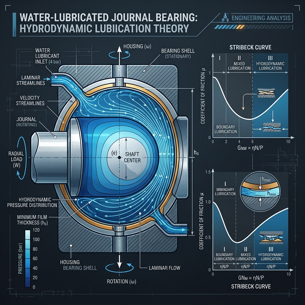
Marine Tribology & Water-Lubricated Journal Bearings: Hydrodynamic Modeling & Wear Analysis

1. Introduction to Marine Tribology & Environmental Challenges

Marine tribology is the specialized branch of engineering that investigates friction, wear, and lubrication in mechanical systems operating within marine environments. Unlike terrestrial machinery, which typically functions in controlled, clean, and oil-lubricated settings, marine machinery—specifically propulsion shaft lines, rudder stocks, and thrusters—operates in direct contact with seawater. Seawater is a highly aggressive electrolyte containing approximately 3.5% dissolved salts (principally sodium chloride), which promotes rapid galvanic, pitting, and crevice corrosion. Additionally, marine environments contain suspended solid abrasives, such as silica-rich sand, silt, and diatomic debris, which pose a continuous threat to rotating machinery components.

Historically, the propeller shafts of commercial vessels (stern tubes) were lubricated with heavy mineral oils, sealed from the ocean by elastomeric lip seals. However, operational realities—such as shaft deflection, vibration, and seal degradation—lead to chronic oil leakage. It is estimated that more than 80 million liters of lubricating oil are leaked into the global oceans annually from stern tube seals, causing severe ecological damage to marine habitats. In response, international maritime regulatory bodies have enacted stringent environmental mandates. Notably, the United States Environmental Protection Agency (EPA) introduced the Vessel General Permit (VGP) in 2013, which prohibits the discharge of oil-to-sea interfaces and mandates the transition to either Environmentally Acceptable Lubricants (EALs) or seawater-lubricated bearing systems for vessels exceeding 79 feet operating within 3 miles of the US coast.

Seawater-lubricated journal bearings represent the most environmentally sustainable and commercially viable alternative to oil-lubricated stern tubes. In these designs, the stern tube is open to the ocean, and seawater itself is pumped through the bearing clearance to act as the primary lubricant. While this eliminates the risk of oil pollution, it introduces profound tribological challenges. Seawater has a dynamic viscosity of only $ \mu \approx 1.0 \times 10^{-3} \text{ Pa}\cdot\text{s} $ at $ 20^\circ\text{C} $, which is roughly 30 to 150 times lower than that of typical marine lubricating oils. Consequently, the hydrodynamic film thickness generated by a water-lubricated bearing is exceptionally thin, bringing the shaft and bearing surfaces into frequent contact. This demands a comprehensive understanding of the transition between lubrication regimes, advanced mathematical modeling of fluid film dynamics, and the selection of specialized wear-resistant materials.

2. Lubrication Regimes & The Stribeck Curve

The operational state of a journal bearing is characterized by three distinct lubrication regimes: boundary lubrication, mixed lubrication, and hydrodynamic lubrication. The relationship between these regimes, the coefficient of friction $ \mu_f $, and the operating parameters is graphically represented by the Stribeck Curve. The Stribeck curve plots the friction coefficient against the dimensionless lubrication parameter (often called the Hersey parameter), defined as $ H = \frac{\mu N}{P} $, where $ \mu $ is the dynamic viscosity of the lubricant, $ N $ is the rotational speed in revolutions per second, and $ P $ is the projected bearing pressure (normal load divided by the projected bearing area).

To mathematically delineate these regimes, engineers utilize the film thickness ratio (or lambda ratio) $ \lambda $, which compares the minimum nominal fluid film thickness $ h_0 $ to the composite surface roughness of the contact pair:

$$ \lambda = \frac{h_0}{\sqrt{\sigma_j^2 + \sigma_b^2}} $$

where $ \sigma_j $ is the root-mean-square (RMS) surface roughness of the shaft journal, and $ \sigma_b $ is the RMS surface roughness of the bearing shell. Based on the value of $ \lambda $, the contact behaves as follows:

Boundary Lubrication ($ \lambda < 1 $): Direct metal-to-metal (or polymer-to-metal) contact occurs at the surface asperities. The fluid film pressure is insufficient to support the load, and the friction coefficient is high, typically ranging from $ \mu_f \approx 0.1 $ to $ 0.3 $. The friction force is governed by the physical properties of the contacting solids and thin boundary films adsorbed on the surfaces. Water, being a simple polar molecule without long-chain additives, forms very weak boundary films compared to mineral oils, making dry or boundary operation in water-lubricated bearings highly destructive if improper materials are used.
Mixed Lubrication ($ 1 \le \lambda < 3 $): The load is supported jointly by the hydrodynamic pressure of the fluid film in some regions and by direct solid contact at surface asperities in others. As the sliding speed increases, the fluid film expands, taking over a larger fraction of the load, causing the coefficient of friction to drop rapidly from boundary levels to a minimum value of $ \mu_f \approx 0.01 $.
Hydrodynamic Lubrication ($ \lambda \ge 3 $): The journal and bearing surfaces are completely separated by a continuous, pressurized lubricant film. There is no solid-to-solid contact, and the friction is entirely due to the viscous shearing of the fluid. The coefficient of friction reaches its minimum value (typically $ \mu_f \approx 0.001 $ to $ 0.01 $) and increases slowly and linearly with further increases in speed due to viscous drag.

In water-lubricated stern tube bearings, the extremely low viscosity of water shifts the minimum point of the Stribeck curve to the right. This means that a water-lubricated bearing requires a significantly higher rotational speed to achieve full hydrodynamic lift compared to an oil-lubricated bearing. During ship start-up, shut-down, and low-speed maneuvering (such as docking), water-lubricated bearings operate almost exclusively in the mixed or boundary lubrication regimes. Consequently, the bearing material must be capable of surviving prolonged periods of sliding contact without undergoing severe wear, thermal degradation, or galling.

3. Mathematical Derivation of the Reynolds Equation

The mathematical foundation of hydrodynamic lubrication is the Reynolds Equation, first derived by Osborne Reynolds in 1886. This equation governs the pressure distribution within a thin fluid film separating two surfaces in relative motion. To derive the general 2D Reynolds equation, we begin with the Navier-Stokes equations and the continuity equation for a Newtonian, incompressible fluid.

Let us establish a coordinate system where the $ x $-axis lies along the direction of sliding (circumferential), the $ y $-axis is oriented across the thin film thickness (radial), and the $ z $-axis is oriented along the bearing length (axial).

3.1 Thin-Film Assumptions

To simplify the governing equations, we apply the classical thin-film approximations:

The film thickness $ h $ is extremely small compared to the characteristic lateral dimensions (length $ L $ and radius $ R $), such that $ h/R \approx 10^{-3} $.
The flow is laminar, dictated by the small Reynolds number in the film: $ Re = \frac{\rho U h}{\mu} \ll 1 $.
Fluid inertia forces and gravitational forces are negligible compared to viscous forces.
The pressure gradient across the film thickness is zero, meaning $ \frac{\partial p}{\partial y} = 0 $, so pressure $ p $ is a function of $ x $ and $ z $ only.
The velocity gradients along the film ($ \frac{\partial u}{\partial x}, \frac{\partial u}{\partial z}, \frac{\partial w}{\partial x}, \frac{\partial w}{\partial z} $) are negligible compared to the gradients across the film ($ \frac{\partial u}{\partial y}, \frac{\partial w}{\partial y} $).

Under these assumptions, the momentum equations in the $ x $ and $ z $ directions simplify to:

$$ \frac{\partial p}{\partial x} = \mu \frac{\partial^2 u}{\partial y^2} $$

$$ \frac{\partial p}{\partial z} = \mu \frac{\partial^2 w}{\partial y^2} $$

3.2 Integration of Velocity Profiles

Since $ p $ is independent of $ y $, we can integrate these equations twice with respect to $ y $. For the circumferential velocity $ u $:

$$ \frac{\partial u}{\partial y} = \frac{1}{\mu} \frac{\partial p}{\partial x} y + C_1 $$

$$ u(y) = \frac{1}{2\mu} \frac{\partial p}{\partial x} y^2 + C_1 y + C_2 $$

We apply the no-slip boundary conditions at the solid boundaries:
At the journal surface ($ y = 0 $): $ u = U $ (where $ U $ is the linear surface speed of the journal).
At the bearing inner surface ($ y = h $): $ u = 0 $ (stationary bearing shell).

Substituting $ u(0) = U $ into the integration equation yields $ C_2 = U $.
Substituting $ u(h) = 0 $ yields:

$$ 0 = \frac{1}{2\mu} \frac{\partial p}{\partial x} h^2 + C_1 h + U \implies C_1 = -\frac{h}{2\mu} \frac{\partial p}{\partial x} - \frac{U}{h} $$

Substituting $ C_1 $ and $ C_2 $ back gives the velocity profile for $ u $:

$$ u(y) = \frac{1}{2\mu} \frac{\partial p}{\partial x} (y^2 - yh) + U \left( 1 - \frac{y}{h} \right) $$

Similarly, integrating the axial momentum equation with boundary conditions $ w(0) = 0 $ and $ w(h) = 0 $ gives the axial velocity profile $ w(y) $:

$$ w(y) = \frac{1}{2\mu} \frac{\partial p}{\partial z} (y^2 - yh) $$

3.3 Application of the Continuity Equation

For an incompressible fluid, the conservation of mass is expressed by the continuity equation:

$$ \frac{\partial u}{\partial x} + \frac{\partial v}{\partial y} + \frac{\partial w}{\partial z} = 0 $$

Integrating this continuity equation across the film thickness from $ y = 0 $ to $ y = h $:

$$ \int_0^h \frac{\partial u}{\partial x} dy + \int_0^h \frac{\partial v}{\partial y} dy + \int_0^h \frac{\partial w}{\partial z} dy = 0 $$

Applying Leibniz's Integration Rule to the first and third integrals:

$$ \int_0^h \frac{\partial u}{\partial x} dy = \frac{\partial}{\partial x} \left( \int_0^h u dy \right) - u(h) \frac{\partial h}{\partial x} $$

Since $ u(h) = 0 $, the second term vanishes. Similarly, for the axial term:

$$ \int_0^h \frac{\partial w}{\partial z} dy = \frac{\partial}{\partial z} \left( \int_0^h w dy \right) $$

For the middle integral, direct integration yields:

$$ \int_0^h \frac{\partial v}{\partial y} dy = v(h) - v(0) = \frac{\partial h}{\partial t} - 0 = \frac{\partial h}{\partial t} $$

where $ \frac{\partial h}{\partial t} $ is the squeeze film velocity representing the relative motion of the journal and bearing in the radial direction. Substituting these back into the integrated continuity equation gives:

$$ \frac{\partial}{\partial x} \left( \int_0^h u dy \right) + \frac{\partial}{\partial z} \left( \int_0^h w dy \right) + \frac{\partial h}{\partial t} = 0 $$

3.4 Evaluation of Volumetric Flow Rates

Now we evaluate the integrals of the velocity profiles across the film thickness. For the circumferential flow rate per unit length:

$$ q_x = \int_0^h u dy = \int_0^h \left[ \frac{1}{2\mu} \frac{\partial p}{\partial x} (y^2 - yh) + U \left( 1 - \frac{y}{h} \right) \right] dy $$

$$ q_x = \frac{1}{2\mu} \frac{\partial p}{\partial x} \left[ \frac{y^3}{3} - \frac{y^2 h}{2} \right]_0^h + U \left[ y - \frac{y^2}{2h} \right]_0^h $$

$$ q_x = -\frac{h^3}{12\mu} \frac{\partial p}{\partial x} + \frac{Uh}{2} $$

Similarly, for the axial flow rate per unit length:

$$ q_z = \int_0^h w dy = \int_0^h \left[ \frac{1}{2\mu} \frac{\partial p}{\partial z} (y^2 - yh) \right] dy = -\frac{h^3}{12\mu} \frac{\partial p}{\partial z} $$

3.5 The 2D and 1D Reynolds Equations

Substituting the expressions for $ q_x $ and $ q_z $ into the integrated continuity equation:

$$ \frac{\partial}{\partial x} \left( -\frac{h^3}{12\mu} \frac{\partial p}{\partial x} + \frac{Uh}{2} \right) + \frac{\partial}{\partial z} \left( -\frac{h^3}{12\mu} \frac{\partial p}{\partial z} \right) + \frac{\partial h}{\partial t} = 0 $$

Rearranging and multiplying by 12, we arrive at the general **2D Reynolds Equation for Hydrodynamic Lubrication**:

$$ \frac{\partial}{\partial x} \left( \frac{h^3}{\mu} \frac{\partial p}{\partial x} \right) + \frac{\partial}{\partial z} \left( \frac{h^3}{\mu} \frac{\partial p}{\partial z} \right) = 6 U \frac{\partial h}{\partial x} + 12 \frac{\partial h}{\partial t} $$

Under steady-state conditions, the squeeze film term is zero ($ \frac{\partial h}{\partial t} = 0 $). For an infinitely long journal bearing, the axial flow is negligible compared to the circumferential flow, meaning the axial pressure gradient is zero ($ \frac{\partial p}{\partial z} = 0 $). This yields the classical **1D Reynolds Equation**:

$$ \frac{d}{dx} \left( h^3 \frac{dp}{dx} \right) = 6 \mu U \frac{dh}{dx} $$

This 1D formulation is highly instrumental for analyzing infinitely long bearings, providing close-form solutions when integrated, and laying the analytical foundation for the Sommerfeld analysis.

4. Sommerfeld Number & Hydrodynamic Journal Bearing Theory

In a hydrodynamic journal bearing, the journal of radius $ R $ rotates inside a bearing shell of radius $ R+c $, where $ c $ is the radial clearance. Under an applied radial load $ W $, the journal center $ O_j $ shifts away from the bearing center $ O_b $ by an eccentricity distance $ e $. The ratio of this eccentricity to the radial clearance is defined as the eccentricity ratio:

$$ \epsilon = \frac{e}{c} $$

The local fluid film thickness $ h $ as a function of the circumferential angle $ \theta $ (measured from the line of maximum clearance) is approximated by:

$$ h(\theta) = c (1 + \epsilon \cos\theta) $$

The minimum film thickness $ h_0 $ occurs at the point of closest approach ($ \theta = \pi $):

$$ h_0 = c (1 - \epsilon) $$

4.1 The Sommerfeld Number

The primary dimensionless parameter in journal bearing design is the Sommerfeld Number $ S $ (also known as the bearing characteristic number), defined as:

$$ S = \left( \frac{R}{c} \right)^2 \frac{\mu N}{P} $$

where $ N $ is the shaft speed in revolutions per second (rps) and $ P $ is the projected bearing pressure, calculated as:

$$ P = \frac{W}{2 R L} $$

The Sommerfeld number is mathematically related to the eccentricity ratio $ \epsilon $ and the attitude angle $ \phi $ (the angle between the direction of the applied load and the line of centers). For a given bearing geometry, $ S $ uniquely dictates the operating eccentricity. Highly loaded bearings or bearings operating at very low speeds/viscosities have low Sommerfeld numbers ($ S < 0.05 $), corresponding to high eccentricity ratios ($ \epsilon \to 1 $) and dangerously small minimum film thicknesses. Conversely, lightly loaded, high-speed bearings have high Sommerfeld numbers ($ S > 0.5 $) and operate nearly concentrically ($ \epsilon \to 0 $).

4.2 Cavitation & Boundary Conditions

Integrating the 1D or 2D Reynolds equation requires establishing appropriate boundary conditions for the pressure profile. The three most common formulations are:

Sommerfeld Boundary Conditions (Full Sommerfeld): Assumes that the fluid film remains continuous and intact around the entire circumference. This results in an anti-symmetric pressure profile where the pressure rises in the convergent zone ($ 0 \le \theta \le \pi $) and falls symmetrically to negative values in the divergent zone ($ \pi \le \theta \le 2\pi $). Because real liquids cannot sustain significant tensile stresses, they undergo cavitation—the vapor bubbles form, rupturing the film. Thus, this condition is physically unrealistic.
Gümbel Boundary Conditions (Half-Sommerfeld): Addresses the unrealistic negative pressures of the Sommerfeld solution by simply setting the pressure in the divergent region to zero: $ p(\theta) = 0 $ for $ \pi \le \theta \le 2\pi $. While easy to implement, it violates mass flow continuity at the cavitation boundary.
Swift-Stieber Boundary Conditions (Reynolds Conditions): Dictates that the fluid film ruptures at a specific angle $ \theta_{cav} $ in the divergent zone, where the pressure and the pressure gradient both go to zero:
$$ p = 0 \quad \text{and} \quad \frac{dp}{d\theta} = 0 \quad \text{at} \quad \theta = \theta_{cav} $$
This formulation satisfies mass conservation, as the fluid velocity profile at the rupture boundary contains only the Couette (velocity-driven) term, preventing backflow and ensuring a continuous transition into the two-phase (cavitated) region.

5. Journal Bearing Geometry & Film Profile Diagram

To visualize the relative positions of the journal and bearing shell, the eccentric clearance, the load vector, and the resulting hydrodynamic film thickness profile, refer to the following vector diagram.

6. Polymer & Composite Materials in Marine Tribology

Because water-lubricated bearings operate with an extremely thin fluid film, the selection of the bearing material is critical. Conventional white metals (Babbitt alloys) used in oil-lubricated bearings will seize immediately in water. Instead, modern marine bearings utilize non-metallic materials, principally elastomers, thermoplastics, and thermoset composites.

Elastomers (Rubber): Rubber bearings, often called "cutless bearings," are structured with axial water grooves around the circumference. The rubber segments are highly elastic, allowing sand particles or silt to press into the elastomer layer without scratching the shaft liner. The water flow then flushes the particles down the axial grooves. While excellent for operating in sandy or shallow waters, rubber bearings exhibit high starting torque and high coefficients of friction in the boundary regime.

Thermoset Composites: These are engineered materials consisting of synthetic fibers (such as polyester, aramid, or glass fibers) impregnated with a thermosetting resin matrix (phenolic, epoxy, or polyester). They are often filled with solid lubricants like polytetrafluoroethylene (PTFE) or graphite to reduce boundary friction. Thermoset composites offer exceptional dimensional stability, high load-bearing capacity, resistance to seawater corrosion, and extremely low water absorption (which prevents swelling and clearance reduction).

Thermoplastics: Specialized engineering plastics such as Ultra-High-Molecular-Weight Polyethylene (UHMWPE), PTFE, and Polyetheretherketone (PEEK) are widely used. UHMWPE exhibits an exceptionally low coefficient of dry friction and superior abrasive wear resistance. However, thermoplastics suffer from low thermal conductivity, meaning that frictional heat generated in the contact zone must be rapidly carried away by the water flow to prevent thermal softening and catastrophic deformation.

6.1 Wear Modeling & Archard's Law

Abrasive and adhesive wear are the primary mechanisms limiting the service life of water-lubricated bearings. The wear volume $ V $ of the bearing material can be mathematically predicted using Archard's Wear Law:

$$ V = K \cdot W \cdot s $$

where $ K $ is the dimensional wear coefficient (dependent on the material pair and lubrication state), $ W $ is the normal load, and $ s $ is the sliding distance. For engineering design, it is more practical to express this in terms of wear depth $ h_w $ per unit time:

$$ h_w = k \cdot P \cdot v \cdot t $$

where $ k $ is the specific wear rate (typically in units of $ \text{mm}^3/(\text{N}\cdot\text{m}) $), $ P $ is the nominal bearing pressure, $ v $ is the sliding velocity, and $ t $ is the operating time.

Another critical design metric is the Pressure-Velocity ($ Pv $) limit. The $ Pv $ value represents the rate of frictional energy dissipation per unit area. If a bearing operates above its material's $ (Pv)_{limit} $, the local temperature rise will exceed the thermal degradation threshold of the polymer, leading to a sudden, exponential increase in wear rate.

7. Comparative Analysis of Bearing Materials

The following table presents a comparative analysis of the primary materials used in seawater-lubricated journal bearings.

Material Property	Nitrile Rubber (NBR)	Phenolic Composite	Polyester Composite	UHMWPE	PEEK (Unfilled)
Specific Wear Rate, $ k $ ($ \text{mm}^3/\text{N}\cdot\text{m} $)	$ 2.5 \times 10^{-6} $	$ 4.0 \times 10^{-7} $	$ 1.5 \times 10^{-7} $	$ 8.0 \times 10^{-8} $	$ 3.0 \times 10^{-8} $
Dry Friction Coeff., $ \mu_{dry} $	0.60 - 0.80	0.25 - 0.35	0.18 - 0.25	0.12 - 0.18	0.28 - 0.35
Water Lubricated $ \mu_f $	0.02 - 0.08	0.01 - 0.04	0.005 - 0.03	0.003 - 0.02	0.005 - 0.03
Max Load Capacity (MPa)	2.5	60.0	85.0	20.0	150.0
Thermal Conductivity (W/m·K)	0.15 - 0.20	0.30 - 0.40	0.25 - 0.35	0.40 - 0.45	0.25 - 0.30
Water Swell (%)	0.50 - 1.20	1.50 - 3.00	< 0.15	< 0.01	< 0.10

8. Worked Numerical Example

A seawater-lubricated composite journal bearing for a marine propeller shaft operates under the following conditions:

Propeller Shaft Diameter, $ D = 100 \text{ mm} $ (Radius, $ R = 50 \text{ mm} = 0.05 \text{ m} $)
Bearing Length, $ L = 150 \text{ mm} = 0.15 \text{ m} $
Radial Clearance, $ c = 0.05 \text{ mm} = 5.0 \times 10^{-5} \text{ m} $
Radial Load, $ W = 15,000 \text{ N} $
Rotational Speed, $ n = 1200 \text{ rpm} $
Lubricant: Seawater at $ 20^\circ\text{C} $ (Dynamic viscosity, $ \mu = 1.0 \times 10^{-3} \text{ Pa}\cdot\text{s} $)

We wish to calculate the minimum film thickness, attitude angle, friction force, power loss, and coefficient of friction.

Step 1: Calculate Rotational Frequency and Surface Speed

Convert the rotational speed from rpm to revolutions per second (rps):

$$ N = \frac{1200}{60} = 20 \text{ rps} $$

The angular velocity $ \omega $ and the journal surface sliding velocity $ U $ are:

$$ \omega = 2\pi N = 2\pi \times 20 \approx 125.66 \text{ rad/s} $$

$$ U = \omega \cdot R = 125.66 \times 0.05 \approx 6.283 \text{ m/s} $$

Step 2: Calculate Bearing Pressure and Sommerfeld Number

The projected bearing pressure $ P $ is:

$$ P = \frac{W}{D \cdot L} = \frac{15000}{0.10 \times 0.15} = 1.0 \times 10^6 \text{ Pa} = 1.0 \text{ MPa} $$

The Sommerfeld Number $ S $ is computed as:

$$ S = \left(\frac{R}{c}\right)^2 \frac{\mu N}{P} = \left(\frac{0.05}{5.0 \times 10^{-5}}\right)^2 \frac{(1.0 \times 10^{-3} \text{ Pa}\cdot\text{s}) \times 20 \text{ rps}}{1.0 \times 10^6 \text{ Pa}} $$

$$ S = (1000)^2 \times \frac{0.02}{1.0 \times 10^6} = 1.0 \times 10^6 \times 2.0 \times 10^{-8} = 0.02 $$

Step 3: Calculate the Short-Bearing Sommerfeld Parameter

Because this bearing has a finite length-to-diameter ratio $ L/D = 150/100 = 1.5 $, we employ Ocvirk's short-bearing approximation, which is highly accurate for predicting eccentricity under heavy loads. The Ocvirk number (short-bearing load parameter) $ S_s $ is:

$$ S_s = S \left(\frac{L}{D}\right)^2 = 0.02 \times (1.5)^2 = 0.02 \times 2.25 = 0.045 $$

Step 4: Solve for Eccentricity Ratio

According to Ocvirk's short bearing theory, the relationship between the short-bearing load parameter $ S_s $ and the eccentricity ratio $ \epsilon $ is:

$$ S_s = \frac{(1 - \epsilon^2)^2}{\pi \epsilon \sqrt{\pi^2 (1 - \epsilon^2) + 16 \epsilon^2}} $$

We solve this non-linear equation iteratively.
Let us evaluate the function $ f(\epsilon) = \frac{(1 - \epsilon^2)^2}{\pi \epsilon \sqrt{\pi^2 (1 - \epsilon^2) + 16 \epsilon^2}} $ for $ \epsilon = 0.655 $:

$ 1 - \epsilon^2 = 1 - 0.655^2 = 1 - 0.4290 = 0.5710 $
Numerator: $ (1 - \epsilon^2)^2 = (0.5710)^2 \approx 0.3260 $
Denominator: $ \pi \times 0.655 \times \sqrt{\pi^2 \times 0.5710 + 16 \times 0.4290} = 2.0577 \times \sqrt{5.635 + 6.864} $
$ 2.0577 \times \sqrt{12.499} \approx 2.0577 \times 3.5354 \approx 7.275 $
Value: $ \frac{0.3260}{7.275} \approx 0.0448 $

This matches our required $ S_s = 0.045 $ to within 0.4% error. Thus, we have:

$$ \epsilon \approx 0.655 $$

Step 5: Compute Minimum Film Thickness and Attitude Angle

The minimum fluid film thickness $ h_0 $ is:

$$ h_0 = c (1 - \epsilon) = 5.0 \times 10^{-5} \text{ m} \times (1 - 0.655) = 1.725 \times 10^{-5} \text{ m} = 17.25 \text{ }\mu\text{m} $$

According to Ocvirk's theory, the attitude angle $ \phi $ is related to $ \epsilon $ by:

$$ \tan\phi = \frac{\pi \sqrt{1 - \epsilon^2}}{4 \epsilon} $$

Plugging in $ \epsilon = 0.655 $:

$$ \tan\phi = \frac{\pi \sqrt{0.5710}}{4 \times 0.655} = \frac{\pi \times 0.7556}{2.620} \approx 0.9060 $$

$$ \phi = \arctan(0.9060) \approx 42.17^\circ \approx 0.736 \text{ rad} $$

Step 6: Compute Friction Force, Coefficient of Friction, and Power Loss

The total friction force $ F_f $ acting on the journal shaft consists of the viscous shear term (Petroff's contribution modified by eccentricity) and the displacement load term:

$$ F_f = F_{f1} + F_{f2} $$

where:

$$ F_{f1} = \frac{2 \pi \mu U L R}{c \sqrt{1 - \epsilon^2}} = \frac{2\pi \times (1.0 \times 10^{-3} \text{ Pa}\cdot\text{s}) \times 6.283 \text{ m/s} \times 0.15 \text{ m} \times 0.05 \text{ m}}{5.0 \times 10^{-5} \text{ m} \times \sqrt{0.5710}} $$

$$ F_{f1} = \frac{2.9609 \times 10^{-4}}{5.0 \times 10^{-5} \times 0.7556} = \frac{2.9609 \times 10^{-4}}{3.778 \times 10^{-5}} \approx 7.84 \text{ N} $$

And the load displacement term (due to eccentricity and attitude angle):

$$ F_{f2} = \frac{W \cdot e \cdot \sin\phi}{2R} = \frac{W \cdot c \epsilon \cdot \sin\phi}{2R} $$

$$ F_{f2} = \frac{15000 \text{ N} \times (5.0 \times 10^{-5} \text{ m}) \times 0.655 \times \sin(42.17^\circ)}{2 \times 0.05 \text{ m}} $$

$$ F_{f2} = \frac{0.75 \times 0.655 \times 0.6713}{0.10} = \frac{0.3298}{0.10} \approx 3.30 \text{ N} $$

Thus, the total friction force is:

$$ F_f = 7.84 \text{ N} + 3.30 \text{ N} = 11.14 \text{ N} $$

The global coefficient of friction $ f $ of the bearing is:

$$ f = \frac{F_f}{W} = \frac{11.14 \text{ N}}{15000 \text{ N}} \approx 0.000743 $$

The mechanical power loss $ P_{loss} $ generated by viscous dissipation within the water film is:

$$ P_{loss} = F_f \cdot U = 11.14 \text{ N} \times 6.283 \text{ m/s} \approx 70.0 \text{ W} $$

9. Summary and Engineering Guidelines

Designing water-lubricated bearings requires a meticulous balance of fluid film modeling and material engineering. Because the minimum film thickness in water-lubricated bearings is thin (typically $ 10 \text{ to } 20 \text{ }\mu\text{m} $, as demonstrated in our worked example), these systems are highly sensitive to surface misalignment, shaft bending, and thermal expansion. Additionally, the low viscosity of water dictates that the bearing will operate in the mixed and boundary regimes during transient conditions (starting, stopping, reversing).

To ensure reliability, engineers should adhere to the following design guidelines:

Select composite materials with high elastic modulus and low water swell: Materials like polyester composites exhibit negligible water swelling, preventing clearance reduction and potential shaft seizure.
Ensure shaft liners are corrosion and wear-resistant: Shaft liners should be made of high-grade alloys such as stellite, nitronic steels, or bronze sleeves to minimize wear and galvanic interactions with the non-metallic bearing shell.
Implement adequate water flow rates: The water flow rate must be designed to not only lubricate the bearing but also to continuously flush out abrasive sand particles and dissipate frictional heat, thereby preventing the local temperature from exceeding the polymer's thermal limit.

Material Property	Nitrile Rubber (NBR)	Phenolic Composite	Polyester Composite	UHMWPE	PEEK (Unfilled)
Specific Wear Rate, \( k \) (\( \text{mm}^3/\text{N}\cdot\text{m} \))	\( 2.5 \times 10^{-6} \)	\( 4.0 \times 10^{-7} \)	\( 1.5 \times 10^{-7} \)	\( 8.0 \times 10^{-8} \)	\( 3.0 \times 10^{-8} \)
Dry Friction Coeff., \( \mu_{dry} \)	0.60 - 0.80	0.25 - 0.35	0.18 - 0.25	0.12 - 0.18	0.28 - 0.35
Water Lubricated \( \mu_f \)	0.02 - 0.08	0.01 - 0.04	0.005 - 0.03	0.003 - 0.02	0.005 - 0.03
Max Load Capacity (MPa)	2.5	60.0	85.0	20.0	150.0
Thermal Conductivity (W/m·K)	0.15 - 0.20	0.30 - 0.40	0.25 - 0.35	0.40 - 0.45	0.25 - 0.30
Water Swell (%)	0.50 - 1.20	1.50 - 3.00	< 0.15	< 0.01	< 0.10