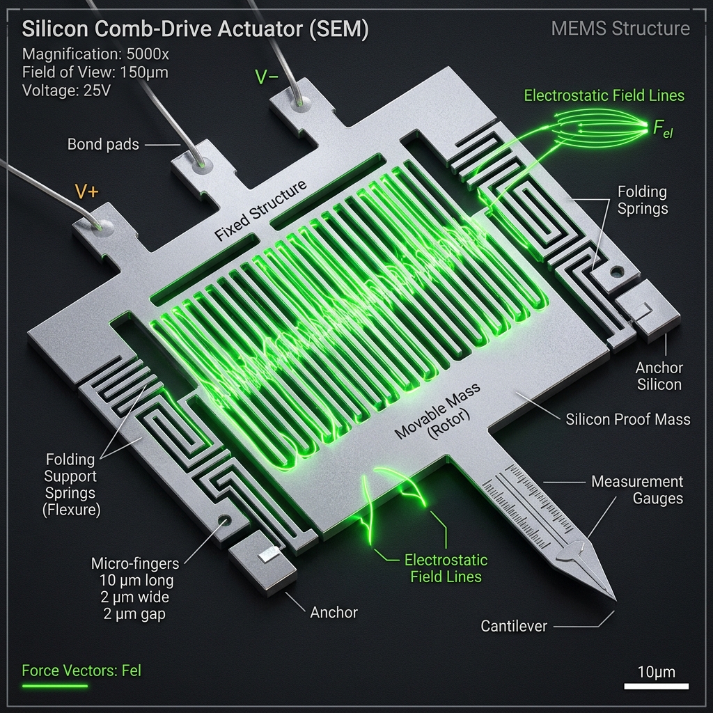
Micro-Electro-Mechanical Systems (MEMS) Multiphysics Modeling

1. Introduction to MEMS Multiphysics Modeling

Micro-Electro-Mechanical Systems (MEMS) represent a major milestone in modern engineering, integrating sensors, actuators, and electronic control circuits on a single silicon substrate. These microscale systems are fabricated using batch-processing techniques derived from the integrated circuit industry, enabling high-precision, high-volume production. By combining micro-sensors, micro-actuators, and microelectronics, MEMS technology enables the creation of smart products that sense, think, act, and communicate. Common applications include accelerometers, gyroscopes, micromirrors, pressure sensors, and microfluidic channels. Modeling these devices is challenging because of the microscale physics involved, which differ significantly from macroscale mechanics.

The necessity of multiphysics modeling in MEMS arises from the fact that physical phenomena are tightly coupled at the microscale. During operation, a MEMS device is rarely governed by a single physical domain. For example, in an electrostatic actuator, an applied voltage creates an electric field that exerts a mechanical force on a movable structure, causing it to deform. This deformation in turn alters the electric field, establishing a two-way electro-mechanical coupling. In addition, the movement of the structure is damped by the surrounding gas, representing a fluid-structure interaction known as squeeze-film damping. Furthermore, if current flows through the structure, Joule heating occurs, leading to temperature gradients and thermal stresses, which affect the mechanical properties and cause thermal expansion (electro-thermo-mechanical coupling). Thus, multiphysics modeling is necessary for design and optimization.

As structural dimensions shrink from the macroscale to the microscale, physical forces scale differently. This scaling behavior can be analyzed as a function of the characteristic length L. Volume-related forces, such as gravity and inertia, scale as L^3. Conversely, surface-related forces, such as electrostatics, surface tension, and viscous drag, scale as L^2 or L^1. Let us analyze the scaling of the electrostatic force versus the gravitational force. If all dimensions scale down by s, and the voltage is scaled down by s to maintain a constant electric field (constant field scaling), the electrostatic force scales as s^2, while the gravitational force scales as s^3. The ratio of electrostatic force to gravitational force scales as s^-1. As size shrinks (s -> 0), the ratio approaches infinity, indicating that electrostatic forces are much stronger than gravity at the microscale, making them ideal for actuation.

Silicon is the primary structural material for MEMS due to its excellent mechanical and electrical properties. Single-crystal silicon (SCS) is an anisotropic material with high yield strength, no mechanical hysteresis, and a Young's modulus that depends on crystallographic orientation. Polycrystalline silicon (polysilicon) is widely used for surface micromachining and is isotropic on average, with a Young's modulus of approximately 160 to 170 GPa. Other materials include silicon dioxide (often used as a sacrificial layer or electrical insulator), silicon nitride (used for membranes and structural layers due to its high dielectric strength and chemical inertness), and various metals (gold, aluminum, copper) for electrical contacts and reflective surfaces. Residual stress, which arises during thin-film deposition, is a critical concern, as it can cause warping or buckling of suspended microstructures.

2. Electrostatic Actuation Principles

Electrostatic actuation operates on the principle of Coulomb attraction between oppositely charged plates. The simplest model of an electrostatic actuator is a parallel-plate capacitor, consisting of a fixed bottom electrode and a movable top electrode separated by a dielectric medium (typically air or vacuum). When a voltage V is applied between these two plates, an electric field is established in the gap. The distribution of the electrostatic potential $ \Phi $ within the gap is governed by Poisson's equation, which is derived from Gauss's law of electromagnetism:

$$ \nabla \cdot (\epsilon \nabla \Phi) = -\rho_e $$

where $ \epsilon $ is the permittivity of the dielectric medium and $ \rho_e $ is the free charge density in the gap. In the absence of free space charge within the gap, this governing equation simplifies directly to Laplace's equation:

$$ \nabla^2 \Phi = 0 $$

For a simplified one-dimensional parallel-plate actuator where the gap distance g is much smaller than the length and width of the plates, the potential variation along the thickness axis z is linear. Integrating Laplace's equation $ \frac{d^2 \Phi}{dz^2} = 0 $ with boundary conditions $ \Phi(0) = 0 $ and $ \Phi(g) = V $ yields:

$$ \Phi(z) = V \frac{z}{g} $$

The corresponding homogeneous electric field E between the plates is given by the negative gradient of the potential:

$$ E = -\frac{d\Phi}{dz} = -\frac{V}{g} $$

The total electrostatic energy $ U_e $ stored in the capacitor at a given gap g and applied voltage V can be expressed as a function of the capacitance C:

$$ U_e = \frac{1}{2} C V^2 $$

For a parallel-plate configuration with plate area A and gap g, the nominal capacitance is $ C = \frac{\epsilon A}{g} $. Substituting this into the energy equation yields:

$$ U_e = \frac{\epsilon A V^2}{2 g} $$

To derive the electrostatic force $ F_e $ acting on the movable plate, we must consider the thermodynamic work balance of the electro-mechanical system under constant voltage control. When the movable plate undergoes an incremental displacement $ dg $, the external voltage source does electrical work $ dW_{source} = V dQ = V^2 dC $ to maintain a constant potential. The change in the stored electrostatic energy is $ dU_e = \frac{1}{2} V^2 dC $. The mechanical work done by the electrostatic force is $ dW_{mech} = F_e dg $. Applying the principle of conservation of energy, the mechanical work must equal the net energy input from the source minus the increase in stored energy:

$$ dW_{mech} = dW_{source} - dU_e $$

$$ F_e dg = V^2 dC - \frac{1}{2} V^2 dC = \frac{1}{2} V^2 dC $$

$$ F_e = \frac{1}{2} V^2 \frac{dC}{dg} $$

Differentiating the capacitance $ C = \frac{\epsilon A}{g} $ with respect to g gives $ \frac{dC}{dg} = -\frac{\epsilon A}{g^2} $. Substituting this derivative back into the force expression yields the fundamental formula for the attractive electrostatic force:

$$ F_e = -\frac{\epsilon A V^2}{2 g^2} $$

The negative sign indicates that the force is attractive, acting to reduce the gap g between the plates. In reality, the electric field lines do not terminate abruptly at the plate edges but bulge outward into the surrounding medium. These fringing field effects increase the effective capacitance and force, particularly for narrow plates. To account for this, analytical corrections are employed. One widely accepted formulation is Palmer's formula, which defines the capacitance per unit length of a plate of width W and thickness t separated by a gap g as:

$$ C_{fringe} = \frac{\epsilon W}{g} \left[ 1 + \frac{g}{\pi W} \left( 1 + \ln\left( \frac{2\pi W}{g} \right) \right) \right] $$

This correction factor is crucial for high-fidelity modeling, as ignoring fringing fields can lead to significant underestimation of the electrostatic forces in microscale structures.

Figure 1: Schematic of a 1D Parallel-Plate Electrostatic Actuator

3. Pull-In Instability and Analytical Derivations

A defining characteristic of voltage-controlled electrostatic actuators is the pull-in instability, a non-linear phenomenon where the electrostatic force overcomes the mechanical restoring force, causing the movable member to snap down and collapse onto the fixed electrode. To analyze this stability limit, we utilize a one-dimensional lumped-parameter model. The actuator is modeled as a movable plate of mass m supported by a linear elastic spring with stiffness constant k. The movable plate is suspended above a parallel fixed plate. Let the initial gap under zero applied voltage be $ g_0 $. When a voltage V is applied, the movable plate deflects by a distance x towards the fixed electrode, reducing the current gap to $ g = g_0 - x $. The dynamic equation of motion of this single-degree-of-freedom system is written as:

$$ m \ddot{x} + b \dot{x} + k x = \frac{\epsilon A V^2}{2 (g_0 - x)^2} $$

where b is the damping coefficient. Under static equilibrium conditions, the velocity and acceleration terms vanish, reducing the governing equation to a balance between the mechanical restoring force $ F_s = k x $ and the electrostatic attraction force $ F_e $:

$$ k x = \frac{\epsilon A V^2}{2 (g_0 - x)^2} $$

Figure 2: Animated Simulation of Electrostatic Pull-In Collapse

To determine the stability of the equilibrium points, we examine the net force function $ F_{net}(x, V) = F_e - F_s = \frac{\epsilon A V^2}{2 (g_0 - x)^2} - k x $. An equilibrium state is stable if a small perturbation away from the state results in a restoring force that pushes the system back. Mathematically, this stability condition requires that the derivative of the net force with respect to the displacement is negative, or equivalently, that the stiffness of the mechanical spring exceeds the gradient of the electrostatic force:

$$ \frac{\partial F_{net}}{\partial x} < 0 \implies \frac{\partial F_e}{\partial x} < \frac{\partial F_s}{\partial x} $$

Differentiating the force expressions with respect to x yields:

$$ \frac{\partial F_{s}}{\partial x} = k $$

$$ \frac{\partial F_e}{\partial x} = \frac{\epsilon A V^2}{(g_0 - x)^3} $$

Thus, the stability limit, which defines the onset of pull-in, occurs when the electrostatic force gradient exactly equals the mechanical spring constant:

$$ k = \frac{\epsilon A V^2}{(g_0 - x_c)^3} $$

where $ x_c $ represents the critical displacement at the threshold of instability. To find this critical displacement, we divide the static force balance equation by the stability limit equation:

$$ \frac{k x_c}{k} = \frac{ \frac{\epsilon A V^2}{2 (g_0 - x_c)^2} }{ \frac{\epsilon A V^2}{(g_0 - x_c)^3} } $$

Simplifying this ratio yields a remarkably elegant and fundamental result:

$$ x_c = \frac{1}{2} (g_0 - x_c) $$

$$ 2 x_c = g_0 - x_c \implies 3 x_c = g_0 $$

$$ x_c = \frac{1}{3} g_0 $$

This derivation demonstrates that under voltage control, a parallel-plate electrostatic actuator can undergo stable static deflection up to a maximum of exactly one-third of the initial gap. Any attempt to deflect the plate further by increasing the voltage results in a loss of stability. To find the pull-in voltage $ V_{pi} $ corresponding to this critical state, we substitute the expression for the critical displacement $ x_c = \frac{1}{3} g_0 $ back into the static equilibrium equation:

$$ k \left( \frac{1}{3} g_0 \right) = \frac{\epsilon A V_{pi}^2}{2 \left( g_0 - \frac{1}{3} g_0 \right)^2} $$

$$ \frac{1}{3} k g_0 = \frac{\epsilon A V_{pi}^2}{2 \left( \frac{2}{3} g_0 \right)^2} $$

$$ \frac{1}{3} k g_0 = \frac{\epsilon A V_{pi}^2}{2 \left( \frac{4}{9} g_0^2 \right)} = \frac{9 \epsilon A V_{pi}^2}{8 g_0^2} $$

Solving this equation for the pull-in voltage $ V_{pi} $ yields the famous analytical formula:

$$ V_{pi} = \sqrt{\frac{8 k g_0^3}{27 \epsilon A}} $$

This instability can be characterized in the phase space using bifurcation theory. The system undergoes a saddle-node bifurcation at $ V = V_{pi} $. For any voltage below the pull-in limit, there are two distinct equilibrium solutions: a stable node at a lower deflection and an unstable saddle at a higher deflection. As the voltage increases, these two points merge. At the pull-in voltage, they coalesce into a single unstable saddle-node. Beyond this voltage, no real equilibrium solutions exist, and the trajectory of the movable plate in the phase space accelerates dynamically toward the fixed plate. Interestingly, if the actuator is operated under charge control rather than voltage control, the pull-in instability is suppressed. Because the charge Q is fixed, the voltage varies as $ V = \frac{Q}{C} = \frac{Q(g_0 - x)}{\epsilon A} $. The electrostatic force is then $ F_e = \frac{Q^2}{2 \epsilon A} $, which is independent of the displacement x. Consequently, a stable force balance exists for all deflections up to the full initial gap $ g_0 $.

4. Squeeze-Film Damping and Micro-Gas Dynamics

In microscale devices, the dynamics of moving parts are heavily influenced by the surrounding fluid medium. Squeeze-film damping is the primary energy dissipation mechanism in structures where a thin gas film is trapped between two close, parallel surfaces moving relative to each other. As the surfaces approach, the gas is compressed and forced to flow outward through the narrow boundary. Because of the gas's viscosity, a pressure gradient develops within the gap, generating a net reaction force that opposes the motion. At the microscale, gas flow cannot always be treated as a continuous fluid. The transition from continuum to rarefied flow is characterized by the dimensionless Knudsen number Kn, defined as the ratio of the molecular mean free path $ \lambda $ of the gas to the characteristic gap distance g:

$$ Kn = \frac{\lambda}{g} $$

Figure 3: Dynamic Simulation of Squeeze-Film Gas Damping

At standard atmospheric pressure and temperature, the mean free path of air is approximately 68 nm. For a typical MEMS gap of 2 microns, the Knudsen number is 0.034. Based on the value of Kn, the flow is classified into four distinct regimes: the continuum regime (Kn < 0.01), the slip flow regime (0.01 < Kn < 0.1), the transition regime (0.1 < Kn < 10), and the free molecular flow regime (Kn > 10). For slip flow and transition regimes, the non-equilibrium effects at the boundaries (velocity slip) must be incorporated. This is commonly achieved by defining an effective viscosity $ \mu_{eff} $ that decreases as the Knudsen number increases. A widely used empirical formulation is Veijola's model:

$$ \mu_{eff} = \frac{\mu_0}{1 + 9.638 Kn^{1.159}} $$

where $ \mu_0 $ is the dynamic viscosity under ambient continuum conditions.

The pressure distribution p(x,y,t) within the squeeze film is modeled using the compressible Reynolds equation, which is derived from the Navier-Stokes equations by invoking the thin-film approximation (assuming the gap height h is much smaller than the lateral dimensions of the plates) and neglecting fluid inertia terms. The general compressible Reynolds equation is written as:

$$ \frac{\partial}{\partial x} \left( p h^3 \frac{\partial p}{\partial x} \right) + \frac{\partial}{\partial y} \left( p h^3 \frac{\partial p}{\partial y} \right) = 12 \mu_{eff} \frac{\partial (p h)}{\partial t} $$

This is a highly non-linear partial differential equation. To obtain analytical insight, we linearize the equation by assuming small-amplitude harmonic oscillations of the plate. We express the pressure and gap height as perturbations around their nominal values:

$$ p(x,y,t) = p_a + \Delta p(x,y,t) $$

$$ h(t) = h_0 + z_0 e^{i \omega t} $$

where $ p_a $ is the ambient atmospheric pressure, $ h_0 $ is the initial gap, $ z_0 $ is the oscillation amplitude (such that $ z_0 \ll h_0 $), $ \Delta p $ is the pressure perturbation (with $ \Delta p \ll p_a $), and $ \omega $ is the excitation frequency. Substituting these perturbation expressions into the Reynolds equation and neglecting higher-order terms yields the linearized Reynolds equation:

$$ \nabla^2 (\Delta p) = \frac{12 \mu_{eff}}{p_a h_0^2} \left( p_a \frac{\partial h}{\partial t} + h_0 \frac{\partial (\Delta p)}{\partial t} \right) $$

The behavior of the linearized system is governed by the dimensionless Squeeze Number $ \sigma $, which represents the ratio of the viscous compression time to the oscillation period:

$$ \sigma = \frac{12 \mu_{eff} \omega L^2}{p_a h_0^2} $$

where L is the characteristic lateral length of the plate. The value of the squeeze number dictates the nature of the fluid reaction force. When the squeeze number is low ($ \sigma \ll 1 $), which occurs at low frequencies, the gas has sufficient time to escape from the edges of the plate. In this regime, the pressure perturbation is in phase with the velocity of the plate, and the gas acts primarily as a viscous damper, dissipating energy. When the squeeze number is high ($ \sigma \gg 1 $), which occurs at high frequencies, the gas is trapped beneath the plate and cannot escape. In this case, the gas is compressed elastically, acting as a pneumatic spring. The pressure perturbation is in phase with the displacement, and energy dissipation is minimized. In multiphysics modeling, this frequency-dependent transition between spring-like and damper-like behavior must be modeled by extracting the frequency-dependent damping and spring coefficients.

5. Micro-Cantilever Beam Mechanics

Suspended beams, such as micro-cantilevers and fixed-fixed bridges, are structural building blocks in many MEMS sensors and actuators. The mechanics of these micro-beams are governed by the Euler-Bernoulli beam theory, which assumes that the cross-sections of the beam remain plane and perpendicular to the neutral axis during bending. The dynamic behavior of a micro-beam with Young's modulus E, density $ \rho $, cross-sectional area $ A_c $, and moment of inertia I is described by the partial differential equation:

$$ E I \frac{\partial^4 w(x,t)}{\partial x^4} + \rho A_c \frac{\partial^2 w(x,t)}{\partial t^2} = q(x,t) $$

where w(x,t) is the transverse deflection of the beam at position x and time t, and q(x,t) is the external distributed load per unit length. For an electrostatically actuated beam, the load is non-uniform and depends non-linearly on the local deflection. Assuming a parallel-ground plane configuration with an applied voltage V and initial gap $ g_0 $, the distributed electrostatic force per unit length is:

$$ q(x) = \frac{\epsilon W V^2}{2 (g_0 - w(x))^2} $$

where W is the width of the beam. This non-linear coupling between deflection and electrostatic loading prevents closed-form analytical solutions for static deflection. Instead, numerical approximations like the finite element method or the Galerkin variational method must be used, where the deflection is expanded as a sum of mechanical mode shapes.

To analyze the dynamic characteristics of the beam under zero external load, we set q(x,t) = 0 and assume a harmonic solution $ w(x,t) = \phi(x) e^{i \omega t} $. This reduces the equation to an eigenvalue problem for the mode shapes $ \phi(x) $:

$$ \frac{d^4 \phi(x)}{dx^4} - \beta^4 \phi(x) = 0 $$

where the spatial eigenvalue $ \beta $ is related to the natural frequency $ \omega $ by $ \beta^4 = \frac{\rho A_c \omega^2}{E I} $. The general solution for the mode shape is:

$$ \phi(x) = A \cosh(\beta x) + B \sinh(\beta x) + C \cos(\beta x) + D \sin(\beta x) $$

For a cantilever beam of length L that is clamped at x = 0 and free at x = L, the boundary conditions are:

$$ \phi(0) = 0, \quad \phi'(0) = 0 $$

$$ \phi''(L) = 0, \quad \phi'''(L) = 0 $$

Applying these boundary conditions yields the characteristic transcendental equation for the eigenvalues:

$$ \cos(\beta L) \cosh(\beta L) = -1 $$

The roots of this equation correspond to the discrete natural modes of the cantilever. The first root, which defines the fundamental resonant mode, is $ \beta_1 L \approx 1.8751 $. The fundamental natural frequency $ \omega_1 $ is then:

$$ \omega_1 = \frac{1.8751^2}{L^2} \sqrt{\frac{E I}{\rho A_c}} = \frac{1.8751^2 t}{L^2} \sqrt{\frac{E}{12 \rho}} $$

Figure 4: Dynamic Cantilever Beam Resonance Modes and Stress Distributions

where t is the beam thickness. When an electrostatic voltage V is applied to the beam, the electrostatic force gradient alters the effective stiffness of the structure. Because the electrostatic force increases as the gap decreases, its gradient acts as a negative spring stiffness. This phenomenon is known as electrostatic spring softening. The effective stiffness $ k_{eff} $ of the micro-beam decreases as the voltage increases:

$$ k_{eff}(V) = k_m - k_e(V) $$

where $ k_m $ is the pure mechanical stiffness and $ k_e(V) = \frac{\partial F_e}{\partial w} $ is the electrostatic stiffness. As a result, the fundamental natural frequency of the beam shifts downward with applied voltage according to:

$$ \omega_0(V) = \omega_0 \sqrt{1 - \left( \frac{V}{V_{pi}} \right)^2} $$

This electrostatic frequency tuning is a critical design tool in MEMS resonators and filters, enabling post-fabrication adjustment of the operational frequency.

6. Electro-Thermo-Mechanical (ETM) Coupling

Electro-thermo-mechanical (ETM) actuators represent another vital class of MEMS devices, operating on the principle of thermal expansion induced by electrical Joule heating. Unlike electrostatic actuators, which require high voltages but consume minimal power, thermal actuators utilize lower voltages and high currents to generate large forces. The multiphysics modeling of an ETM system involves three coupled physical domains: electrical conduction, thermal transport, and structural mechanics. The coupling is sequential and two-way: electrical current flow generates heat, the heat generates temperature fields, the temperature fields induce mechanical strains and stresses, and the resulting deformation and temperature changes alter the electrical and thermal properties.

The electrical domain is governed by current continuity. The current density vector $ \mathbf{J} $ is related to the electrical potential V and the temperature-dependent electrical conductivity $ \sigma_{elec}(T) $ by Ohm's law:

$$ \mathbf{J} = -\sigma_{elec}(T) \nabla V $$

$$ \nabla \cdot (\sigma_{elec}(T) \nabla V) = 0 $$

The electrical energy dissipated per unit volume due to resistive losses is the Joule heat source term $ Q_{Joule} $:

$$ Q_{Joule} = \mathbf{J} \cdot E = \sigma_{elec}(T) |\nabla V|^2 $$

This heat source enters the transient heat transfer equation, which governs the temperature distribution T within the microstructure:

$$ \rho c_p \frac{\partial T}{\partial t} - \nabla \cdot (k_{th}(T) \nabla T) = Q_{Joule} - q_{loss} $$

where $ \rho $ is the material density, $ c_p $ is the specific heat capacity, and $ k_{th} $ is the thermal conductivity. In microscale structures, heat loss $ q_{loss} $ to the surrounding air and substrate is extremely significant due to the high surface-to-volume ratio. Convective and radiative heat losses from the surfaces are modeled as boundary conditions. More importantly, heat conduction through the narrow air gap to the underlying silicon substrate represents a dominant heat sink. This is typically modeled as a distributed heat loss term proportional to the temperature difference:

$$ q_{loss} = S \frac{k_{air}}{g} (T - T_{substrate}) $$

where $ k_{air} $ is the thermal conductivity of air, g is the gap height, $ T_{substrate} $ is the substrate temperature (usually assumed to be constant at ambient room temperature), and S is a shape factor that accounts for fringing heat flux from the sides of the micro-beam.

The mechanical domain is coupled to the thermal domain through thermal strain. The total strain tensor $ \epsilon $ is the sum of the elastic strain $ \epsilon_{el} $ and the thermal expansion strain $ \epsilon_{th} $:

$$ \epsilon = \epsilon_{el} + \epsilon_{th} $$

$$ \epsilon_{th} = \alpha (T - T_0) \mathbf{I} $$

where $ \alpha $ is the coefficient of thermal expansion (CTE), $ T_0 $ is the stress-free reference temperature, and $ \mathbf{I} $ is the identity tensor. The mechanical stresses are related to the elastic strains by Hooke's law. In a fully constrained beam, such as a fixed-fixed bridge, the thermal expansion is restricted, leading to the development of axial compressive stresses:

$$ \sigma_{thermal} = -E \alpha (T - T_0) $$

If the average temperature rise exceeds a critical threshold, the compressive stress will trigger mechanical buckling. In electro-thermal actuators like V-beam (chevron) actuators, the beams are designed with a pre-bend angle. As the temperature rises, the expansion of the beams causes them to bend outward in a predetermined direction, translating axial thermal expansion into lateral actuation displacement. Resolving these coupled ETM physics requires iterative numerical solvers, where the electrical, thermal, and mechanical equations are solved sequentially or monolithically until convergence is reached.

7. MEMS Actuation Mechanisms: Comparative Analysis

To design an effective MEMS device, engineers must select the most appropriate actuation mechanism based on the application's constraints. The table below provides a comprehensive comparison of the four primary MEMS actuation methods: Electrostatic (both parallel-plate and comb-drive configurations), Thermal (such as V-beam actuators), Piezoelectric, and Electromagnetic.

Actuation Mechanism	Force Density	Stroke / Displacement	Operating Voltage	Power Consumption	Bandwidth / Speed	Key Disadvantage
Electrostatic (Parallel Plate)	Medium (high at small gaps)	Small (limited to 1/3 of gap)	Medium (10V - 100V)	Near Zero (negligible leakage)	High (up to several MHz)	Pull-in instability limits travel
Electrostatic (Comb Drive)	Low	Large (up to dozens of microns)	High (50V - 150V)	Near Zero (leakage only)	High (tens of kHz)	Lateral instability (shorting risk)
Electro-Thermal (V-Beam)	Very High	Medium (up to 20 microns)	Low (5V - 15V)	High (milliwatts to watts)	Low (limited by thermal time constant)	High power draw, thermal fatigue
Piezoelectric (PZT film)	High	Small (unless bimorph design)	Low to Medium (5V - 30V)	Low (capacitive load)	Very High (up to GHz)	Hysteresis, complex thin-film deposition
Electromagnetic	Medium	Very Large (hundreds of microns)	Low (1V - 5V)	Medium to High (Joule heating in coils)	Medium (hundreds of Hz)	Difficult integration of micro-coils/magnets

8. Worked Numerical Example: Parallel-Plate and Comb-Drive Actuators

Let us solve a detailed, exam-style engineering problem to calculate the mechanical, electrical, and stability characteristics of two fundamental MEMS actuators: a parallel-plate actuator and a comb-drive actuator. The calculations are presented step-by-step using KaTeX for formulas and values.

Part A: Parallel-Plate Actuator Pull-In Voltage

Consider a parallel-plate electrostatic actuator with the following physical parameters:

- Plate Area: $ A = 1.5 \times 10^{-7} \text{ m}^2 $ (corresponding to a plate of $ 500 \ \mu\text{m} \times 300 \ \mu\text{m} $)

- Initial Air Gap: $ g_0 = 3.0 \ \mu\text{m} = 3.0 \times 10^{-6} \text{ m} $

- Mechanical Spring Constant: $ k = 15.0 \text{ N/m} $

- Permittivity of Free Space: $ \epsilon_0 = 8.854 \times 10^{-12} \text{ F/m} $ (assuming air in the gap)

We wish to find the critical deflection $ x_c $ and the pull-in voltage $ V_{pi} $.

Step 1: Calculate the critical deflection prior to pull-in

Using the derivation from Section 3, the critical deflection before instability occurs is exactly one-third of the initial gap:

$$ x_c = \frac{1}{3} g_0 = \frac{3.0 \times 10^{-6} \text{ m}}{3} = 1.0 \times 10^{-6} \text{ m} = 1.0 \ \mu\text{m} $$

Step 2: Calculate the pull-in voltage

We substitute the system parameters into the pull-in voltage formula:

$$ V_{pi} = \sqrt{\frac{8 k g_0^3}{27 \epsilon_0 A}} $$

$$ V_{pi} = \sqrt{\frac{8 \times 15.0 \text{ N/m} \times (3.0 \times 10^{-6} \text{ m})^3}{27 \times 8.854 \times 10^{-12} \text{ F/m} \times 1.5 \times 10^{-7} \text{ m}^2}} $$

$$ V_{pi} = \sqrt{\frac{120.0 \times 2.7 \times 10^{-17}}{3.58587 \times 10^{-17}}} $$

$$ V_{pi} = \sqrt{\frac{3.24 \times 10^{-15}}{3.58587 \times 10^{-17}}} = \sqrt{90.3547} \approx 9.51 \text{ V} $$

Thus, the pull-in voltage for this parallel-plate actuator is $ 9.51 \text{ V} $, and the plate collapses if deflected beyond $ 1.0 \ \mu\text{m} $.

Part B: Comb-Drive Actuator Drive Force and Lateral Instability

Now consider a polysilicon MEMS comb-drive actuator with a folded-beam suspension. The design parameters are:

- Number of Movable Fingers: $ N = 60 $

- Finger Height (Thickness): $ t = 12.0 \ \mu\text{m} = 1.2 \times 10^{-5} \text{ m} $

- Finger Initial Overlap: $ L_0 = 15.0 \ \mu\text{m} = 1.5 \times 10^{-5} \text{ m} $

- Gap between Fingers: $ g = 1.5 \ \mu\text{m} = 1.5 \times 10^{-6} \text{ m} $

- Suspension Beam Length: $ L_s = 180.0 \ \mu\text{m} = 1.8 \times 10^{-4} \text{ m} $

- Suspension Beam Width: $ w_s = 2.5 \ \mu\text{m} = 2.5 \times 10^{-6} \text{ m} $

- Young's Modulus of Polysilicon: $ E = 165.0 \text{ GPa} = 1.65 \times 10^{11} \text{ N/m}^2 $

- Permittivity of Free Space: $ \epsilon_0 = 8.854 \times 10^{-12} \text{ F/m} $

We want to compute: 1) the mechanical spring constants in the drive direction (x) and lateral direction (y); 2) the electrostatic force and deflection at an applied voltage of 50 V; 3) the lateral pull-in voltage at this state.

Step 1: Calculate the suspension spring constants

The shuttle is supported by a folded-beam suspension with four beams. The mechanical stiffness in the drive direction $ k_x $ (weak axis bending) is:

$$ k_x = \frac{2 E t w_s^3}{L_s^3} $$

$$ k_x = \frac{2 \times (1.65 \times 10^{11}) \times (1.2 \times 10^{-5}) \times (2.5 \times 10^{-6})^3}{(1.8 \times 10^{-4})^3} $$

$$ k_x = \frac{3.96 \times 10^6 \times 1.5625 \times 10^{-17}}{5.832 \times 10^{-12}} = \frac{6.1875 \times 10^{-11}}{5.832 \times 10^{-12}} \approx 10.61 \text{ N/m} $$

The stiffness in the lateral direction $ k_y $ (strong axis bending, where thickness is t and width is $ w_s $) is given by swapping $ w_s $ and t:

$$ k_y = \frac{2 E w_s t^3}{L_s^3} = k_x \left( \frac{t}{w_s} \right)^2 $$

$$ k_y = 10.6096 \times \left( \frac{1.2 \times 10^{-5}}{2.5 \times 10^{-6}} \right)^2 = 10.6096 \times 4.8^2 = 10.6096 \times 23.04 \approx 244.45 \text{ N/m} $$

Step 2: Calculate the drive force and displacement at V = 50 V

A comb-drive actuator with N movable fingers has 2N active electrostatic gaps. The electrostatic force generated along the drive direction x is constant and independent of x:

$$ F_x = N \frac{\epsilon_0 t V^2}{g} $$

$$ F_x = 60 \times \frac{8.854 \times 10^{-12} \text{ F/m} \times 1.2 \times 10^{-5} \text{ m} \times (50.0 \text{ V})^2}{1.5 \times 10^{-6} \text{ m}} $$

$$ F_x = 60 \times 8.854 \times 10^{-12} \times 8 \times 2500 $$

$$ F_x = 60 \times 8.854 \times 10^{-12} \times 2.0 \times 10^4 = 1.0625 \times 10^{-5} \text{ N} = 10.625 \ \mu\text{N} $$

The displacement x in the drive direction under this force is:

$$ x = \frac{F_x}{k_x} = \frac{1.06248 \times 10^{-5} \text{ N}}{10.6096 \text{ N/m}} \approx 1.0014 \times 10^{-6} \text{ m} \approx 1.00 \ \mu\text{m} $$

Step 3: Calculate the lateral pull-in voltage

The lateral pull-in voltage depends on the current finger overlap $ L_0 + x $. At V = 50 V, $ x \approx 1.00 \ \mu\text{m} $. The overlap is $ L_{total} = L_0 + x = 15.0 \ \mu\text{m} + 1.00 \ \mu\text{m} = 16.0 \ \mu\text{m} = 1.6 \times 10^{-5} \text{ m} $.

The lateral pull-in voltage formula derived in Section 3 is:

$$ V_{pi, lateral} = \sqrt{\frac{k_y g^3}{2 N \epsilon_0 t (L_0 + x)}} $$

$$ V_{pi, lateral} = \sqrt{\frac{244.45 \text{ N/m} \times (1.5 \times 10^{-6} \text{ m})^3}{2 \times 60 \times 8.854 \times 10^{-12} \text{ F/m} \times 1.2 \times 10^{-5} \text{ m} \times 1.6 \times 10^{-5} \text{ m}}} $$

$$ V_{pi, lateral} = \sqrt{\frac{244.45 \times 3.375 \times 10^{-18}}{120 \times 8.854 \times 10^{-12} \times 1.92 \times 10^{-10}}} $$

$$ V_{pi, lateral} = \sqrt{\frac{8.25019 \times 10^{-16}}{2.03996 \times 10^{-19}}} = \sqrt{4044.29} \approx 63.60 \text{ V} $$

At V = 50 V, the system is stable because $ 50 \text{ V} < 63.60 \text{ V} $. However, if the voltage is increased to $ 63.60 \text{ V} $, the transverse electrostatic force gradient will exceed the lateral spring restoring capability, causing the fingers to snap sideways into contact with each other. This lateral pull-in limits the maximum operating stroke of the comb-drive.

9. Conclusion and Design Guidelines

In summary, Micro-Electro-Mechanical Systems (MEMS) design is fundamentally a multiphysics modeling challenge. Mechanical, electrostatic, fluidic, and thermal domains cannot be treated in isolation because of the tight coupling at the microscale. As structural dimensions decrease, the surface-to-volume ratio increases, making electrostatic forces and squeeze-film gas effects dominant. For electrostatic actuators, the pull-in voltage represents a critical mechanical instability that limits stable static deflection to one-third of the initial gap. For comb-drives, while travel in the actuation direction is linear and free of pull-in, lateral pull-in imposes a strict upper bound on voltage and stroke, which must be carefully accounted for by designing suspensions with high lateral stiffness.

Squeeze-film damping is essential for predicting the dynamic response of MEMS devices, transitioning from a pure damping loss at low frequencies to an elastic gas spring at high frequencies. When designing these systems, modeling the non-equilibrium flow rarefaction using effective viscosity models is mandatory. In addition, electro-thermo-mechanical actuators offer large forces and low voltage operation but suffer from high power consumption and slow thermal response times, presenting clear engineering trade-offs. By combining analytical formulations, KaTeX derivations, and comprehensive computational tools like finite element analysis (FEA), mechanical engineers can confidently navigate these complex coupled phenomena to design the next generation of robust micro-transducers.