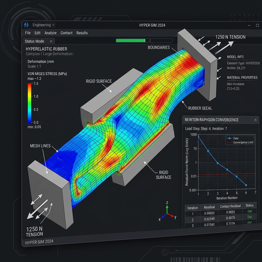
Nonlinear FEA Formulations & Hyperelastic Material Models
1. Introduction to Nonlinear Solid Mechanics
In classical linear elastic solid mechanics, the assumption of infinitesimal deformations is central. This assumption implies that the displacements of material points are very small compared to the characteristic dimensions of the body, and that the rotations are negligible. Consequently, the distinction between the undeformed (reference) configuration and the deformed configuration is ignored, and the kinematic relations are linearized. However, many engineering applications involve situations where these assumptions fail. Structural systems such as high-clearance cables, flexible aerospace structures, soft tissues, elastomeric bearings, and metal forming processes undergo large displacements and rotations, necessitating a transition to Nonlinear Finite Element Analysis (FEA).
Nonlinearities in solid mechanics are broadly classified into three categories:
- Geometric Nonlinearity: Arises when the deformation of the structure significantly changes its shape, orientation, or boundary conditions, such that the equations of equilibrium must be formulated in the deformed configuration. Examples include large deflections, large rotations, and structural buckling.
- Material (Constitutive) Nonlinearity: Occurs when the relationship between stress and strain is nonlinear, history-dependent, or inelastic. Examples include hyperelasticity (elastomers), plasticity (metals yielding), viscoelasticity, and damage mechanics.
- Boundary/Contact Nonlinearity: Arises when the boundary conditions change during the analysis, typical of contact problems where the area of contact depends on the applied load and deformation.
This article focuses on the mathematical formulation of geometric nonlinearity through finite strain kinematics, coupled with hyperelastic material models (specifically Neo-Hookean and Mooney-Rivlin formulations), culminating in the derivation of the tangent stiffness matrix for the Newton-Raphson solution procedure.
2. Kinematics of Finite Deformation
Let us define a body occupying a reference configuration \(\Omega_0\) at time \(t = 0\). A material point in this configuration is identified by its position vector \(\mathbf{X}\). Due to external loading, the body deforms, and at a subsequent time \(t\), it occupies a deformed configuration \(\Omega\). The material point \(\mathbf{X}\) moves to a new spatial position \(\mathbf{x}\). The motion of the body is described by a continuous mapping function:
The displacement vector \(\mathbf{u}\) of the material point is the difference between its spatial and material coordinates:
To analyze local deformation, we introduce the key kinematic quantity, the Deformation Gradient Tensor \(\mathbf{F}\), defined as the gradient of the motion map with respect to the reference coordinates:
In terms of the displacement vector, the deformation gradient is expressed as:
where \(\mathbf{I}\) is the second-order identity tensor, and \(\nabla_X \mathbf{u}\) is the displacement gradient tensor. In index notation, \(F_{iJ} = \delta_{iJ} + \frac{\partial u_i}{\partial X_J}\). The determinant of \(\mathbf{F}\), denoted by \(J\), represents the local volume ratio:
To ensure physical admissibility (no interpenetration of matter), we require \(J > 0\). The deformation gradient \(\mathbf{F}\) contains information about both rotation and stretch. According to the Polar Decomposition Theorem, \(\mathbf{F}\) can be uniquely decomposed into an orthogonal tensor \(\mathbf{R}\) (representing pure rotation, where \(\mathbf{R}^T\mathbf{R} = \mathbf{I}\)) and a symmetric positive-definite tensor representing pure stretch:
where \(\mathbf{U}\) is the right (material) stretch tensor, and \(\mathbf{V}\) is the left (spatial) stretch tensor. To eliminate the rotation component \(\mathbf{R}\), we define the Right Cauchy-Green Deformation Tensor \(\mathbf{C}\):
Similarly, the Left Cauchy-Green Deformation Tensor \(\mathbf{b}\), also known as the Finger tensor, is defined as:
While \(\mathbf{C}\) and \(\mathbf{b}\) characterize deformation, they do not vanish in the undeformed state (where \(\mathbf{F} = \mathbf{I}\), and thus \(\mathbf{C} = \mathbf{b} = \mathbf{I}\)). To define a strain measure that is zero in the absence of deformation, we introduce the Green-Lagrange Strain Tensor \(\mathbf{E}\):
Expanding this in terms of displacement gradients yields:
In component form:
The quadratic term \((\nabla_X \mathbf{u})^T \nabla_X \mathbf{u}\) represents the geometric nonlinearity. When displacement gradients are small, this term is neglected, recovering the classical infinitesimal strain tensor \(\boldsymbol{\varepsilon} = \frac{1}{2}(\nabla \mathbf{u} + (\nabla \mathbf{u})^T)\).
3. Stress Measures in Finite Deformations
In finite deformation theory, we must distinguish between different configurations when defining traction and stress. The most common stress measures are the Cauchy stress, the First Piola-Kirchhoff stress, and the Second Piola-Kirchhoff stress.
Cauchy Stress Tensor \(\boldsymbol{\sigma}\)
The Cauchy Stress Tensor \(\boldsymbol{\sigma}\) (also called true stress) represents the force per unit deformed area. It is defined in the current (deformed) configuration. The traction vector \(\mathbf{t}\) on a surface element with normal \(\mathbf{n}\) in the current configuration is given by:
Conservation of angular momentum dictates that the Cauchy stress tensor is symmetric: \(\boldsymbol{\sigma} = \boldsymbol{\sigma}^T\).
First Piola-Kirchhoff Stress Tensor \(\mathbf{P}\)
The First Piola-Kirchhoff (PK1) Stress Tensor \(\mathbf{P}\) (nominal stress) relates the forces in the deformed configuration to the areas in the reference configuration. If \(\mathbf{t}_0\) is the traction vector in the reference configuration (force divided by reference area) and \(\mathbf{N}\) is the normal to the reference surface:
The relationship between the Cauchy stress and the PK1 stress is derived using Nanson's formula for surface areas, yielding:
Note that the PK1 stress is generally asymmetric (\(\mathbf{P} \neq \mathbf{P}^T\)) because it has one leg in the deformed configuration and one in the reference configuration. This asymmetry makes it computationally inconvenient for many finite element formulations.
Second Piola-Kirchhoff Stress Tensor \(\mathbf{S}\)
To obtain a symmetric stress tensor defined entirely in the reference configuration, we pull back the force vector from the current configuration to the reference configuration. The resulting Second Piola-Kirchhoff (PK2) Stress Tensor \(\mathbf{S}\) is defined as:
Since \(\boldsymbol{\sigma}\) is symmetric, it is straightforward to show that \(\mathbf{S}\) is also symmetric (\(\mathbf{S} = \mathbf{S}^T\)). The PK2 stress does not have an easy direct physical interpretation as a force-per-area vector; however, it is work-conjugate to the Green-Lagrange strain tensor \(\mathbf{E}\), which makes it highly valuable in Lagrangian formulations.
4. Constitutive Modeling & Hyperelasticity
A material is defined as hyperelastic if there exists a scalar-valued function \(\psi\), representing the strain energy density per unit reference volume, from which the stress state can be derived. The strain energy density \(\psi\) must depend only on the deformation gradient \(\mathbf{F}\) (or equivalents) and must satisfy the principle of material frame-indifference, meaning it is invariant under superposed rigid body rotations. This requirement is satisfied if \(\psi\) depends on \(\mathbf{F}\) only through the right Cauchy-Green tensor \(\mathbf{C}\):
Using the Clausius-Duhem inequality for an isothermal process, the rate of work done by the PK2 stress must equal the rate of change of strain energy:
Since this inequality must hold for all arbitrary deformation rates \(\dot{\mathbf{C}}\), we obtain the fundamental hyperelastic constitutive relation:
For isotropic hyperelastic materials, \(\psi\) can be written as a function of the three principal invariants of \(\mathbf{C}\):
where the invariants are defined as:
Applying the chain rule, the PK2 stress is expressed as:
The fourth-order material tangent elasticity tensor \(\mathbb{C}\), which relates increments of PK2 stress to increments of Green-Lagrange strain, is obtained by differentiating \(\mathbf{S}\) with respect to \(\mathbf{C}\):
5. The Neo-Hookean Material Model
The Neo-Hookean model is the simplest hyperelastic model, extending Hooke's law to finite deformations. It is based on the statistical thermodynamics of polymer chain networks.
Incompressible Neo-Hookean Model
For an incompressible material, the volume ratio must remain constant, i.e., \(J = 1\), which implies \(I_3 = 1\). The strain energy density function is:
where \(\mu\) is the shear modulus. To account for the incompressibility constraint, we introduce a Lagrange multiplier \(p\) (interpretable as hydrostatic pressure), yielding the modified potential:
Differentiating with respect to \(\mathbf{C}\) (noting that \(\frac{\partial J}{\partial \mathbf{C}} = \frac{1}{2} J \mathbf{C}^{-1}\)), we get the PK2 stress:
Pushing this stress forward to the current configuration, the Cauchy stress \(\boldsymbol{\sigma}\) is:
where \(\mathbf{b} = \mathbf{F}\mathbf{F}^T\) is the left Cauchy-Green tensor.
Compressible Neo-Hookean Model
For compressible formulations, we must add a volumetric strain energy term that penalizes volume changes and ensures that \(\psi \to \infty\) as \(J \to 0\) (infinite resistance to compression) or \(J \to \infty\). A common formulation is:
where \(\mu\) and \(\lambda\) are the Lamé parameters in the infinitesimal limit. Let us derive the PK2 stress step-by-step using:
First, we know that:
And since \(J = (I_3)^{1/2}\), we have:
Now, applying these derivatives to our strain energy function:
To find the Cauchy stress, we push forward the PK2 stress:
Noting that \(\mathbf{F}\mathbf{F}^T = \mathbf{b}\) and \(\mathbf{F}\mathbf{C}^{-1}\mathbf{F}^T = \mathbf{F}(\mathbf{F}^{-1}\mathbf{F}^{-T})\mathbf{F}^T = \mathbf{I}\), this simplifies to:
This matches the expected stress state and reduces exactly to the linear elastic Hooke's law under infinitesimal strains (where \(J \approx 1 + \text{tr}(\boldsymbol{\varepsilon})\) and \(\mathbf{b} - \mathbf{I} \approx 2\boldsymbol{\varepsilon}\)).
6. The Mooney-Rivlin Material Model
The Mooney-Rivlin model is a phenomenological hyperelastic model that extends the Neo-Hookean model by including the second invariant of the right Cauchy-Green tensor. It provides a more accurate representation of rubber-like materials, particularly under shear and moderate tension.
Incompressible Mooney-Rivlin Model
The strain energy potential for a two-parameter incompressible Mooney-Rivlin material is:
where \(C_{10}\) and \(C_{01}\) are material constants. The shear modulus in the infinitesimal limit is given by \(\mu = 2(C_{10} + C_{01})\). The PK2 stress for this model is obtained by differentiating \(\psi\) with respect to \(\mathbf{C}\):
Pushing forward to the current configuration, we obtain the Cauchy stress tensor:
The inclusion of the \(\mathbf{b}^{-1}\) term allows the model to capture the non-linear shear response and the difference in tensile/compressive behavior of elastomers far better than the Neo-Hookean model.
7. Nonlinear Finite Element Formulations
In nonlinear solid mechanics, there are two primary formulations for describing the deformation of a body: the Total Lagrangian (TL) formulation and the Updated Lagrangian (UL) formulation.
- Total Lagrangian Formulation: All kinematic and static variables are referred to the initial (undeformed) configuration \(\Omega_0\) at time \(t=0\). This is particularly convenient for hyperelastic materials because the material parameters and strain energy potentials are naturally defined with respect to the reference state.
- Updated Lagrangian Formulation: All variables are referred to the current (deformed) configuration at the beginning of the load step. While mathematically equivalent to the TL formulation, the UL formulation is often preferred in plastic flow and large shear problems.
In the TL formulation, the weak form of the momentum balance equation (principle of virtual work) is formulated over the reference volume \(V_0\) as:
where \(\delta \mathbf{u}\) is the virtual displacement field, \(\delta \mathbf{E}\) is the virtual Green-Lagrange strain tensor, \(\mathbf{b}_0\) is the body force vector per unit reference volume, and \(\mathbf{t}_0\) is the traction vector on the reference boundary \(\Gamma_0\).
To discretize the weak form, the continuous displacement and virtual displacement fields are interpolated using shape functions \(N_a(\mathbf{X})\) and nodal values:
The virtual Green-Lagrange strain \(\delta \mathbf{E}\) is related to the virtual nodal displacements by:
where \(\mathbf{B}_{L, a}\) is the linear-in-increment strain-displacement matrix (which depends on the current displacements \(\mathbf{u}\)). Substituting these discretizations into the weak form leads to the discrete residual equation at each node:
where the internal force vector at node \(a\) is:
8. Newton-Raphson Solution Procedure and Tangent Stiffness Matrix
Because \(\mathbf{f}_{int}\) is a highly nonlinear function of the displacements \(\mathbf{u}\) (due to both geometric and material nonlinearities), the residual equation \(\mathbf{R}(\mathbf{u}) = \mathbf{0}\) cannot be solved directly. Instead, we employ an iterative solver such as the Newton-Raphson method.
Suppose we have an estimate \(\mathbf{u}^k\) of the displacement field at iteration \(k\). We perform a Taylor series expansion of the residual around \(\mathbf{u}^k\) and neglect higher-order terms:
This yields the linear system:
where the Tangent Stiffness Matrix \(\mathbf{K}_T\) is defined as:
The displacement is then updated: \(\mathbf{u}^{k+1} = \mathbf{u}^k + \Delta \mathbf{u}\). This loop is repeated until the residual norm \(\|\mathbf{R}\|\) and displacement increment norm \(\|\Delta \mathbf{u}\|\) fall below specified tolerances.
By taking the directional derivative of the internal force vector, we decompose the tangent stiffness matrix into two physically distinct matrices:
-
Material Stiffness Matrix \(\mathbf{K}_{M, ab}\): Represents the stiffness due to the constitutive properties of the material. It depends on the fourth-order material tangent elasticity tensor \(\mathbb{C}\):
$$ \mathbf{K}_{M, ab} = \int_{V_0} \mathbf{B}_{L, a}^T \mathbb{C} \mathbf{B}_{L, b} \, dV_0 $$
-
Geometric (Initial Stress) Stiffness Matrix \(\mathbf{K}_{G, ab}\): Accounts for the change in the structural stiffness due to existing stresses acting on the changing geometry. It is independent of the material tangent elasticity tensor and depends only on the current PK2 stress tensor \(\mathbf{S}\):
$$ \mathbf{K}_{G, ab} = \left( \int_{V_0} \nabla N_a \cdot \mathbf{S} \nabla N_b \, dV_0 \right) \mathbf{I} $$where \(\mathbf{I}\) is the Identity tensor. The geometric stiffness matrix is what allows nonlinear FEA to model phenomena like tension-stiffening in cables and structural buckling.
9. Comparison of Hyperelastic Material Models
Hyperelastic material models differ in their strain energy potentials and parameters, making them suitable for different classes of materials and ranges of deformation. The table below provides a comparative analysis of the most widely used hyperelastic models.
10. Material Deformation & Newton-Raphson Path Visualization
To visualize the kinematics of finite deformation, the physics of hyperelastic constitutive models, and the numerical convergence of nonlinear finite element analysis, three detailed animated diagrams are presented below.
10.1 Hyperelastic plate mesh deformation
This animation shows a 2D/3D rubber specimen mesh under tension stretching and contracting, with color contours changing from blue (zero stress) to red showing stress concentration. The original reference shape \(\Omega_0\) is shown as a dashed outline. Because of hyperelastic incompressibility, the specimen contracts laterally as it is pulled vertically. Notice the high stress concentration factor \(K_t \approx 3\) developing at the horizontal sides of the hole.
10.2 Newton-Raphson iteration path
This step-by-step animation illustrates the convergence of a Newton-Raphson solver to find the equilibrium solution for the nonlinear residual equation \(R(u) = 0\). Starting from an initial guess \(u_0\), each step calculates the tangent line (representing the tangent stiffness \(K_T\)), projects it to the zero-residual line to find the next displacement guess, drops down to evaluate the new residual, and repeats. This iterative path demonstrates the characteristic quadratic convergence rate as it closes in on the solution \(u^*\).
10.3 Hyperelastic stress-strain curve comparison
This plot dynamically traces the uniaxial tensile stress-strain behavior of three hyperelastic models: Neo-Hookean (indigo), Mooney-Rivlin (teal), and Ogden (rose). A sweeping vertical line tracks coordinates on all three curves. The Neo-Hookean and Mooney-Rivlin models are suitable for moderate stretch, while the Ogden model captures the physical strain-stiffening (J-shape) characteristic of elastomers at large stretch.
11. Worked Numerical Example
Problem Description:
A hyperelastic block has reference dimensions \(L_0 = 100\text{ mm}\), \(W_0 = 50\text{ mm}\), and \(H_0 = 50\text{ mm}\). It is subjected to uniaxial tension along its length (the 1-direction), causing a stretch ratio of \(\lambda_1 = 1.5\). The material behaves as an incompressible Neo-Hookean solid with an initial shear modulus \(\mu = 2.0\text{ MPa}\). Assuming that the loading is quasi-static, the deformation is homogeneous, and the lateral surfaces are traction-free, compute:
- The deformation gradient tensor \(\mathbf{F}\) and the right Cauchy-Green deformation tensor \(\mathbf{C}\).
- The Green-Lagrange strain tensor \(\mathbf{E}\).
- The strain energy density \(\psi\) and total strain energy stored in the block.
- The hydrostatic pressure \(p\) from the boundary conditions.
- The Second Piola-Kirchhoff (PK2) stress tensor \(\mathbf{S}\).
- The Cauchy stress tensor \(\boldsymbol{\sigma}\).
- The engineering (nominal) stress and force required to hold the block in tension.
- The 1D tangent modulus in terms of stretch, \(E_{tan} = \frac{d\sigma_{11}}{d\lambda_1}\).
Step 1: Deformation Gradient Tensor \(\mathbf{F}\) and Right Cauchy-Green Tensor \(\mathbf{C}\)
Due to the incompressibility constraint, the determinant of the deformation gradient must be unity, \(J = \det(\mathbf{F}) = \lambda_1 \lambda_2 \lambda_3 = 1\). For uniaxial tension, the symmetry of the block dictates that the lateral stretches are equal: \(\lambda_2 = \lambda_3\). Therefore:
Given \(\lambda_1 = 1.5\), the lateral stretches are:
The deformation gradient tensor \(\mathbf{F}\) in the principal coordinate system is:
The right Cauchy-Green deformation tensor \(\mathbf{C} = \mathbf{F}^T \mathbf{F}\) is:
Step 2: Green-Lagrange Strain Tensor \(\mathbf{E}\)
The Green-Lagrange strain tensor is calculated as:
Step 3: Strain Energy Density and Total Strain Energy
The first invariant of \(\mathbf{C}\) is:
The strain energy density \(\psi\) for an incompressible Neo-Hookean material is:
The volume of the block in the reference configuration is:
Since the deformation is homogeneous, the total stored strain energy \(U\) is:
Step 4: Hydrostatic Pressure \(p\)
The Cauchy stress for an incompressible Neo-Hookean material is:
Since \(\mathbf{F}\) is diagonal, \(\mathbf{b} = \mathbf{F}\mathbf{F}^T = \mathbf{C}\). Thus, the Cauchy stress components are:
The lateral surfaces of the block are traction-free, which means the lateral true stresses must be zero: \(\sigma_{22} = \sigma_{33} = 0\). Using this boundary condition:
Substituting the known values:
Step 5: Second Piola-Kirchhoff (PK2) Stress Tensor \(\mathbf{S}\)
The PK2 stress tensor is given by:
Calculating the components:
Substituting \(\lambda_1 = 1.5\) and \(\mu = 2.0\text{ MPa}\):
Thus, the PK2 stress tensor is:
Step 6: Cauchy Stress Tensor \(\boldsymbol{\sigma}\)
The Cauchy stress tensor components are:
Thus, the Cauchy stress tensor is:
As a verification, check the relation \(\sigma_{11} = S_{11} \lambda_1^2 = 1.4074 \cdot 2.25 = 3.1667\text{ MPa}\). This matches perfectly.
Step 7: Nominal Stress and Applied Force
The nominal/engineering stress \(P_{11}\) is the force divided by the initial cross-sectional area:
The initial cross-sectional area is:
The force \(F_{tens}\) required to pull and hold the block at this stretch is:
Step 8: 1D Tangent Modulus \(E_{tan}\)
The 1D tangent modulus represents the rate of change of Cauchy stress with respect to stretch under uniaxial loading:
Substituting \(\mu = 2.0\text{ MPa}\) and \(\lambda_1 = 1.5\):
Note that in the limit of small strains (where \(\lambda_1 \to 1\)), the tangent modulus approaches \(E_{tan} \to 3\mu = 6.0\text{ MPa}\), which matches the exact relationship \(E = 2\mu(1+\nu)\) for an incompressible linear elastic solid where Poisson's ratio \(\nu = 0.5\).