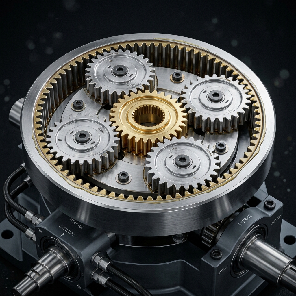
Analytical and Numerical Design of Epicyclic Gear Trains for High-Torque Robotic Actuators

Section 1: Introduction and Kinematic Fundamentals of Epicyclic Gear Trains

In the realm of advanced robotics, particularly in legged locomotion, collaborative manipulation, and space exploration, the actuator serves as the primary bottleneck for system performance. Robotic joint actuation demands an extremely challenging set of performance characteristics: high torque-to-weight ratio (torque density), high torsional stiffness, minimal backlash, exceptional shock load capacity, and bidirectional mechanical transparency (backdrivability). To meet these requirements, designers typically couple high-performance, frameless, brushless DC (BLDC) motors with high-ratio speed reducers. Among the various transmission technologies available, Epicyclic Gear Trains (EGTs)—commonly referred to as planetary gearboxes—stand out due to their coaxial arrangement, compact volume, and outstanding power-sharing capabilities. This section establishes the fundamental kinematic topology, mobility constraints, and structural classifications of EGTs, positioning them within the landscape of modern robotic actuator design.

1.1 Architectural Topology and Kinematic Components

An epicyclic gear train is a coaxial mechanism consisting of three primary coaxial components, supplemented by a set of orbiting planet gears. The architectural topology is characterized by the following elements:

• Sun Gear (S): A centrally located external gear that rotates about the system's main longitudinal axis. It acts as the inner boundary of the gear train and is typically coupled directly to the high-speed input shaft (e.g., the motor rotor).
• Ring Gear (R) or Annulus: An internally toothed gear concentric with the sun gear. The ring gear forms the outer radial boundary of the mechanism and is frequently fixed to the actuator housing to act as a ground plane, though it can remain free to rotate in differential and coupled configurations.
• Planet Gears (P): A set of externally toothed pinions located radially between the sun and ring gears. The planets mesh simultaneously with the sun gear (external-external contact) and the ring gear (external-internal contact).
• Planet Carrier (C): A structural frame that rotates about the central axis. The carrier supports the shafts (planet pins) on which the planet gears spin. The carrier coordinates the orbital motion of the planets and is usually the low-speed, high-torque output member of the transmission.

The meshing kinematics of an EGT are fundamentally distinct from parallel-shaft gear trains. In a standard parallel-shaft arrangement, the teeth of two meshing gears experience external-external contact. This contact type features convex-to-convex geometry, which results in relatively small contact areas (under load) and consequently high Hertzian contact pressures. In contrast, the planet-to-ring mesh in an EGT is an external-internal mesh, characterized by convex-to-concave contact. This geometry is conformal, meaning the shapes of the meshing teeth curve in the same direction. This conformal contact dramatically increases the contact area at the pitch point, significantly reducing local contact stresses and allowing the ring-planet mesh to support substantially higher loads than a comparable external gear pair.

To ensure smooth operation, the teeth of the sun, planet, and ring gears must share the same module ($m$, in metric units) or diametral pitch ($P_d$, in US customary units) and pressure angle ($\phi$). The geometric constraint dictates that the center distance from the central axis to the planet pin ($a$) must be identical whether calculated from the sun gear or the ring gear. For a simple EGT with spur gears, this yields the fundamental geometric relation:

where $r_s$, $r_p$, and $r_r$ are the pitch radii of the sun, planet, and ring gears, respectively. Expressing these radii in terms of tooth counts ($N = 2r/m$), we obtain:

This tooth count relationship is a necessary condition for concentricity and radial alignment in a simple epicyclic gear train. However, when multiple planet gears are introduced to distribute the torque, additional assembly constraints must be satisfied. If $N_{planets}$ is the number of planet gears distributed symmetrically around the carrier, the planet pin angles are spaced at intervals of $2\pi / N_{planets}$. For the teeth of all planets to mesh simultaneously with the sun and ring gears without binding, the total number of teeth on the sun and ring gears must be an integer multiple of the number of planets:

If this condition is violated, the angular positions of the teeth on the sun and ring gears at the nominal planet locations will be out of phase, preventing assembly of the gear train.

Derivation of the Mesh Phasing Constraint

To understand the origin of the assembly condition, let us derive the constraint from first principles. Consider a simple epicyclic gear train with a sun gear, a ring gear, and $N_{planets}$ planets. Let us place the first planet gear ($P_1$) at an angular position $\theta_1 = 0$. The sun gear and the ring gear are oriented such that their teeth mesh perfectly with $P_1$. Now, we wish to place a second planet gear ($P_2$) at an angular position $\theta_2 = 2\pi / N_{planets}$.

For $P_2$ to slide into place and mesh with the sun and ring gears, the tooth spaces of the sun and ring gears at the angle $\theta_2$ must align with the tooth profiles of $P_2$. The angular pitch of the sun gear is $\theta_p^s = 2\pi / N_s$ and that of the ring gear is $\theta_p^r = 2\pi / N_r$. The angular position of the sun gear tooth space relative to the planet carrier is modulated by its rotation. Let the sun gear be rotated by an angle $\alpha_s$ and the ring gear by an angle $\alpha_r$. The angular positions of the tooth spaces on the sun and ring gears at the position of the second planet pin must correspond to an integer number of pitches.

The phase angle of the sun gear at the position of the second planet pin is:

Similarly, the phase angle of the ring gear at the position of the second planet pin is:

For the planet gear $P_2$ to mesh simultaneously with both the sun and ring gears, the sum of these phase indices must be an integer, which ensures that the tooth geometry of the planet meshes with the relative alignment of the sun and ring teeth. Because the planet gear meshes externally with the sun and internally with the ring, a rotation of the planet gear relates the sun and ring phase positions. Summing the phase values:

Under static assembly, we can define the reference position where the first planet is inserted ($\alpha_s = 0, \alpha_r = 0$). For the second planet to be inserted, the phase sum must be a pure integer:

If this condition is not met, the teeth of the planet gear will clash with the teeth of the sun or ring gears, and the gearbox cannot be assembled without elastic deformation or backlash adjustments.

1.2 Mobility Analysis and Degrees of Freedom

A key analytical step in the design of EGTs is determining the mechanism's mobility, or degrees of freedom (DOF). We evaluate mobility using the planar Chebychev-Kutzbach-Grübler criterion:

where $L$ is the number of links in the system, $J_1$ is the number of joints with one degree of freedom (lower pairs, such as revolute joints), and $J_2$ is the number of joints with two degrees of freedom (higher pairs, such as rolling-sliding contacts at gear meshes).

Consider a simple planetary gear train containing $N_p$ planets. Let us inventory the links and joints:

• Links ($L$): The housing (ground) acts as Link 1. The sun gear ($S$) is Link 2. The carrier ($C$) is Link 3. The ring gear ($R$) is Link 4. Each of the $N_p$ planet gears represents a separate moving link. Therefore, the total number of links is:
  $$ L = 4 + N_p $$
• 1-DOF Joints ($J_1$): There are revolute joints connecting the sun gear to the ground, the carrier to the ground, and the ring gear to the ground. Additionally, each planet gear is connected to the carrier via a revolute joint (the planet pin bearing). This yields:
  $$ J_1 = 3 + N_p $$
• 2-DOF Joints ($J_2$): Each planet gear meshes with the sun gear (one contact point) and the ring gear (one contact point). This gives two higher-pair rolling-sliding contacts per planet:
  $$ J_2 = 2 N_p $$

Substituting these values into the Kutzbach-Grübler mobility equation:

This result presents a classic kinematic paradox. If $N_p = 1$ (a single planet gear), the equation yields $M = 2$, indicating a two-degree-of-freedom mechanism. This is physically correct: if we input rotation to both the sun and the carrier, the ring gear's rotation is uniquely determined. However, if $N_p = 3$ (the industry standard), the formula yields $M = 0$. Mathematically, this implies the mechanism is locked and behaves as a rigid structure. In practice, however, planetary gearboxes with three, four, or even six planets rotate freely with exactly two degrees of freedom.

The discrepancy arises because the Kutzbach-Grübler criterion assumes all constraints are independent and the links are in general spatial arrangements. An EGT has kinematic redundancies (or over-constraints) due to its highly symmetric geometry. The additional planets do not introduce new independent kinematic constraints; rather, they replicate the constraint already imposed by the first planet. They are added purely to split the load and reduce the forces acting on the tooth meshes and bearings.

These redundant constraints make the system statically indeterminate. If the components were perfectly rigid and manufactured with slight errors in concentricity or tooth thickness, the gearbox would jam. To prevent jamming and ensure uniform load sharing among the planets, modern robotic actuators employ floating components (e.g., allowing the sun gear to float radially without a dedicated support bearing, centering itself purely via meshing forces) or introduce structural compliance in the carrier pin mounts.

1.3 Structural Variants and Kinematic Inversions

Because a basic epicyclic gear train has two degrees of freedom ($M = 2$), it can be operated in several different ways. By fixing one of the three primary coaxial members (Sun, Carrier, or Ring) to the ground, we reduce the mobility to $M = 1$, yielding three distinct kinematic inversions. A fourth configuration leaves all three members free to rotate, operating as a differential.

In modern high-torque actuators, more complex structural variants are often required to achieve very high reduction ratios in a single compact stage. A prime example is the Wolfrom compound planetary gear train. The Wolfrom drive consists of a sun gear, a single planet carrier carrying compound (stepped) planet gears, and two ring gears: one fixed to the frame and one serving as the rotating output. The compound planet gears have two coaxial sections with different tooth counts: $P_1$ meshes with the fixed ring $R_1$, and $P_2$ meshes with the rotating output ring $R_2$. Because the tooth counts of the two ring gears and the compound planet sections differ only slightly, the carrier's rotation translates into an extremely small relative rotation of the output ring gear. The Wolfrom configuration allows reduction ratios on the order of 1:100 to 1:500 within a single stage, offering a rigid and backdrivable alternative to strain-wave and cycloidal drives.

1.4 Historical Evolution and Contemporary Robotics Paradigms

The concept of epicyclic gearing has a rich history, dating back to antiquity. The earliest known physical implementation of an epicyclic gear train is the Antikythera Mechanism (circa 150–100 BC), an ancient Greek analog computer used to calculate astronomical positions and cycles. The mechanism employed epicyclic gears to model the non-uniform motion of the moon (due to its elliptical orbit) using a pin-and-slot mechanism embedded within an orbiting gear pair. During the Middle Ages and the Renaissance, epicyclic gearing was reinvented and refined for use in elaborate astronomical clocks, such as those designed by Richard of Wallingford and Giovanni de' Dondi. The Industrial Revolution saw the integration of EGTs into heavy machinery, such as James Watt's sun and planet gear (used to bypass the patent on the simple crank for converting reciprocating steam engine motion to rotary motion) and early automotive differential gearboxes.

In contemporary robotics, the paradigm of actuator design has shifted from high-impedance, highly geared systems to low-impedance, highly dynamic systems. Historically, robotic joints relied almost exclusively on Harmonic Drives (Strain Wave Gears) due to their zero-backlash characteristics and high single-stage reduction ratios (typically 1:50 to 1:160). However, strain wave gears suffer from several distinct disadvantages: they are highly fragile under shock loads, have low torsional stiffness, exhibit significant non-linear torque ripple, and are difficult to backdrive. These properties make them poorly suited for applications involving physical interaction, force control, or impact absorption.

To overcome these limitations, modern robotics has embraced two key design approaches:

1. Quasi-Direct Drives (QDD): Popularized by legged robots (e.g., the MIT Cheetah, Boston Dynamics' Atlas, and various commercial quadruped platforms), QDD actuators couple a high-torque, low-speed motor (typically with a large gap radius and high slot-pole count) to a low-ratio (e.g., 1:5 to 1:10) planetary gearhead. Because the gear ratio is low, the reflected inertia of the motor rotor ($I_{\text{reflected}} = I_{\text{rotor}} \cdot R^2$) remains low, making the joint highly backdrivable and transparent. This allows the robot to sense external forces directly through motor current measurements and absorb high-velocity impacts without damaging the gearbox.
2. High-Torque Custom Epicyclic Reducers: For heavy-duty manipulators, humanoid joints, and robotic exoskeletons requiring higher torque than QDDs can provide, compound epicyclic configurations (such as Wolfrom drives or multi-stage planetary gearboxes) are engineered. These systems offer high torsional stiffness, exceptional torque density, and high shock load tolerance.

This table highlights why planetary gearboxes are the preferred transmission for dynamic robotic applications: they balance high mechanical efficiency, robust shock load resistance, and backdrivability, making them the cornerstone of modern robotic joint design.

Section 2: Mathematical Derivations of Gear Ratios & Willis Formula

Designing an epicyclic gear train requires precise control over the velocity relationships between its members. Because the planets orbit the central axis while spinning on their own shafts, tracking the absolute speeds of the gear teeth is geometrically complex. This section presents three analytical methods to derive speed ratios in EGTs: the relative velocity method, the Willis equation, and the tabular method. Additionally, it provides rigorous derivations for standard planetary configurations and the Wolfrom compound drive.

2.1 Kinematic Fundamentals and Relative Velocity Method

Let us define the absolute angular velocities of the primary components:

• $\omega_s$: Absolute angular velocity of the sun gear.
• $\omega_c$: Absolute angular velocity of the planet carrier.
• $\omega_r$: Absolute angular velocity of the ring gear.
• $\omega_p$: Absolute angular velocity of the planet gear about its own center axis.

We establish a rotating reference frame attached to the carrier $C$. In this frame, the carrier is stationary ($\omega'_c = 0$), and all other components rotate relative to it. The relative angular velocities in the carrier-fixed frame are:

Now, we analyze the contact points between the gear meshes. Let $A$ be the pitch contact point between the sun gear and the planet gear. Since the sun and planet gears mesh externally, their relative linear velocities at point $A$ must be equal in magnitude but opposite in direction in the carrier-fixed frame. The relative linear velocity is:

Substituting the relative angular velocities:

where $N_s$ and $N_p$ are the tooth counts of the sun and planet gears. The negative sign represents the inversion of rotational direction inherent in an external gear mesh.

Next, let $B$ be the pitch contact point between the planet gear and the ring gear. Because the planet and ring gears mesh internally, they rotate in the same direction in the carrier-fixed frame. The relative linear velocity at point $B$ is:

Substituting the relative angular velocities:

Here, the ratio is positive because the mesh is internal, meaning the planet and ring gears rotate in the same direction relative to the carrier.

2.2 Formal Derivation of the Willis Equation

The Willis equation, formulated by Robert Willis in 1841, provides a systematic algebraic tool for solving epicyclic gear kinematics. We derive the Willis equation directly by multiplying the relative velocity ratios from Equation (1) and Equation (2):

Let us define the basic gear train value ($e$) as the speed ratio of the ring gear to the sun gear when the carrier is fixed ($\omega_c = 0$):

Substituting $e$ into our combined relative velocity ratio, we obtain the general form of the Willis Equation:

We can rearrange Equation (3) to solve for the absolute angular velocity of any of the three members. Expanding the equation:

Solving for the carrier speed $\omega_c$:

Substituting the definition of the basic train value $e = - \frac{N_s}{N_r}$ into Equation (4):

Equation (5) is the fundamental velocity relationship for a simple epicyclic gear train. It shows that the carrier speed is a weighted average of the sun and ring gear speeds, where the weights are proportional to their respective tooth counts.

2.3 The Tabular Method

For complex or multi-stage epicyclic gear trains, the relative velocity method can become algebraically cumbersome. The tabular method provides a structured alternative that simplifies tracking relative rotations. The method splits the motion of the gear train into two sequential kinematic steps:

1. Carrier Fixed, Sun Rotates: We lock the carrier ($\omega_c = 0$) and rotate one gear (typically the sun) by a hypothetical number of revolutions, $+x$. We then compute the resulting revolutions of the other gears based on the fixed-carrier gear ratios.
2. Rigid Rotation: We unlock the carrier and rotate the entire gear train (including the carrier) as a single rigid body by $+y$ revolutions. In this step, no teeth slide or mesh relative to each other.

We then sum the rotations from both steps to find the absolute rotation of each component.

To prove that the tabular method is mathematically equivalent to the Willis equation, let us write the absolute angular velocities of the carrier, sun, and ring from the total rotation row of the table:

Substituting Equations (6) and (7) into Equation (8):

This matches the Willis equation exactly. The tabular method is not a different mathematical theory, but a visual ledger for organizing the equations of the relative velocity method.

2.4 Case Studies in Speed Ratio Derivations

Let us apply these kinematic tools to specific planetary gear train configurations.

Case A: Fixed Ring Gear ($\omega_r = 0$, Input Sun, Output Carrier)

This is the standard configuration for planetary gearheads used in robotic actuators. Setting $\omega_r = 0$ in the carrier speed equation (Equation 5):

The gear ratio ($R = \omega_{\text{input}} / \omega_{\text{output}}$) is:

Since $N_r$ is typically larger than $N_s$ (often by a factor of 3 to 5), this configuration provides a significant speed reduction and torque multiplication in a compact space. The output carrier rotates in the same direction as the input sun gear.

Case B: Fixed Sun Gear ($\omega_s = 0$, Input Ring, Output Carrier)

Setting $\omega_s = 0$ in Equation (5):

The gear ratio is:

This configuration provides a lower reduction ratio than the fixed-ring case (typically between 1.2 and 1.5) and is rarely used on its own in robotics, though it is common in multi-stage transmissions.

Case C: Wolfrom Compound Planetary Gear Train

The Wolfrom compound planetary gear train is designed for high-ratio reduction. It features:

• A single carrier ($C$) supporting compound planet gears. Each compound planet has two coaxially joined sections: $P_1$ (with $N_{p1}$ teeth) and $P_2$ (with $N_{p2}$ teeth). Because they are rigidly connected, they rotate at the same speed: $\omega_{p1} = \omega_{p2} = \omega_p$.
• An input sun gear ($S$, with $N_s$ teeth) that meshes with planet section $P_1$.
• A fixed ring gear ($R_1$, with $N_{r1}$ teeth) that meshes with planet section $P_1$.
• A rotating output ring gear ($R_2$, with $N_{r2}$ teeth) that meshes with planet section $P_2$.

We begin by establishing the relative velocity relationships in the carrier-fixed frame. For the first stage (Sun $S$, Planet section $P_1$, Fixed Ring $R_1$, Carrier $C$):

Since the sun gear and planet section $P_1$ mesh externally:

The fixed ring gear $R_1$ meshes internally with planet section $P_1$. Since the ring gear is stationary ($\omega_{r1} = 0$), the relative speed of the ring gear is:

The internal mesh relation yields:

Now, we equate the two expressions for the relative speed of the planet (Equations 9 and 10):

Equation (11) gives the angular velocity of the carrier as a function of the input sun gear speed.

Next, we analyze the second stage (Planet section $P_2$, Rotating Ring $R_2$). In the carrier-fixed frame, the relative velocity of the output ring gear $R_2$ is:

Since planet section $P_2$ meshes internally with ring gear $R_2$, their relative speeds are related by:

Because the planet sections are rigidly joined, $\omega'_{p2} = \omega'_{p1} = \omega_p - \omega_c$. Thus:

We substitute the relative planet speed from Equation (10) into Equation (12):

Finally, we substitute the carrier speed from Equation (11) into Equation (13):

Equation (14) is the general kinematic equation for the Wolfrom compound planetary gear train. The overall transmission ratio $i_{\text{wolfrom}} = \omega_s / \omega_{r2}$ is:

To illustrate the reduction capacity of this system, consider a practical numerical example. We select the following tooth counts for the first stage:

We select $N_{p2} = 39$ for the second stage planet section. To ensure concentricity and correct mesh geometry, both stages must share the same center distance $a$. Assuming a constant module $m$, the center distance constraints are:

Equating $a_1$ and $a_2$ yields:

We substitute these tooth counts ($N_s = 20$, $N_{r1} = 100$, $N_{p1} = 40$, $N_{p2} = 39$, $N_{r2} = 99$) into Equation (15) to calculate the reduction ratio:

The Wolfrom drive achieves an outstanding reduction ratio of 396:1 in a single physical stage. The output ring gear rotates in the same direction as the input sun gear. This compact arrangement is highly rigid, features low backlash, and has a high torque capacity, making it a powerful transmission choice for robotic actuators.

Relative Phasing and Manufacturing Constraints of Compound Planets

While the kinematic analysis of the Wolfrom gear train shows its high gear ratio capability, physical construction introduces a strict manufacturing constraint known as compound planet tooth phasing. In a compound planet gear, the two gear profiles $P_1$ and $P_2$ are cut onto a single, solid piece of metal or are keyed together on a shared shaft. This means that the relative angular orientation (or phase angle) between the teeth of $P_1$ and $P_2$ is fixed.

When assembling the gear train with $N_{planets}$ compound planet gears, each planet must be placed at an angle $\theta_j = 2\pi(j-1)/N_{planets}$. For all planet gears to mesh simultaneously with the sun gear, fixed ring gear $R_1$, and rotating ring gear $R_2$, the relative angular alignment of the teeth on $P_1$ and $P_2$ must be identical across all planets. If the tooth profiles are not cut with identical angular phasing relative to a reference keyway or tooth, the planetary gears cannot be assembled without jamming. Specifically, the required angular phase shift ($\psi$) between the tooth centerlines of the two planet stages is given by:

To avoid custom phasing for each planet—which makes manufacturing extremely difficult—designers must select tooth counts that result in a phase shift of zero, or a phase shift that matches the natural symmetry of the teeth. If $\psi = 0$ or is an integer multiple of the tooth pitch, the compound planets can be identical and assembled at any station. Meeting this constraint requires careful optimization of the tooth counts $N_s$, $N_{r1}$, $N_{p1}$, $N_{p2}$, and $N_{r2}$ during the initial design phase.

Section 3: Torque Distribution, Mechanical Efficiency, & Tooth Contact Stresses

Developing a highly reliable planetary gear train for robotic applications requires a deep understanding of its load distribution, mechanical losses, and stress states. Static kinematic models are insufficient when designing systems subjected to high dynamic loads, shock forces, and continuous thermal cycles. This section presents analytical models for static and dynamic torque distribution, details mechanical efficiency calculations using the virtual power method, and reviews the AGMA standards for bending and contact stress analysis.

3.1 Static and Dynamic Torque Analysis

To determine the internal loads acting on the bearings and gear teeth, we must perform a complete force and torque balance. Let $T_s$, $T_c$, and $T_r$ be the external torques applied to the sun gear, carrier, and ring gear, respectively. Under static equilibrium, the sum of all external torques must equal zero:

Assuming an idealized, lossless system, conservation of energy dictates that the net mechanical power input to the system must equal zero:

We can express the carrier velocity using the fundamental carrier speed relationship (Equation 5):

Substituting this expression into the power equation (Equation 17):

Because the sun and ring gear velocities ($\omega_s$ and $\omega_r$) are kinematically independent in a two-degree-of-freedom system, Equation (18) must hold for all possible speed combinations. Consequently, the coefficients of $\omega_s$ and $\omega_r$ must independently equal zero:

Dividing Equation (20) by Equation (19) yields the static torque ratios:

Equations (21) and (22) show that in an ideal, lossless planetary gear train, the output torque at the carrier is equal to the input torque multiplied by the gear ratio, while the ring gear experiences a reaction torque proportional to the ratio of the ring-to-sun tooth counts.

For dynamic modeling, we must account for the rotational inertias of the gears and carrier. We derive the equations of motion using the Euler-Lagrange formulation. Let $\theta_s$ and $\theta_c$ be the generalized coordinates of the system, representing the rotations of the sun gear and the carrier, respectively. The kinetic energy ($T$) of the planetary gear train is:

where $I_s$, $I_c$, $I_r$, and $I_p$ are the mass moments of inertia of the sun, carrier, ring, and planet gears, $m_p$ is the mass of each planet, and $v_{p,k}$ is the linear velocity of the center of mass of the $k$-th planet gear. The planets are mounted on the carrier at a radial distance $a = r_s + r_p$, so their linear velocity is:

The absolute angular velocity of each planet gear is:

For the common case where the ring gear is fixed ($\theta_r = 0$, $\dot{\theta}_r = 0$), the kinematic constraints allow us to express the kinetic energy solely in terms of the independent coordinate $\theta_s$ (or $\theta_c$, since $\dot{\theta}_c = \dot{\theta}_s \frac{N_s}{N_s + N_r}$). Substituting these relations into Equation (23):

where the equivalent mass moment of inertia reflected to the sun gear ($I_{eq}$) is:

Applying Lagrange's equation ($\frac{d}{dt}(\frac{\partial T}{\partial \dot{\theta}_s}) - \frac{\partial T}{\partial \theta_s} = Q_s$), we obtain the dynamic equation of motion:

where $R = 1 + N_r/N_s$ is the gear ratio and $\eta$ is the mechanical efficiency. Equation (24) is critical for designing closed-loop control algorithms in robotics, as it models the effective inertia and motor torque required during high-acceleration maneuvers.

In a real gearbox, manufacturing variations (such as pitch runout, profile errors, and pin position misalignment) prevent the torque from being shared equally among the planets. To account for this, designers apply a planet load sharing factor, $K_\gamma$. The maximum load transmitted by a single planet is defined as:

For a rigidly supported carrier and sun gear with standard manufacturing tolerances, $K_\gamma$ typically ranges from 1.15 to 1.30. By allowing the sun gear to float radially, the gear mesh forces naturally center the sun gear between the planets, balancing the load and reducing $K_\gamma$ to approximately 1.05 to 1.10.

3.2 Power Flow and Efficiency Formulations

Calculating the efficiency of an EGT is challenging because the power transmitted through the system is split into two distinct paths:

1. Coupling Power (Carrier Power): Power transmitted by the rigid rotation of the components with the carrier. Because there is no relative motion or sliding between the teeth during this motion, coupling power is transmitted with 100% mechanical efficiency.
2. Mesh Power (Relative Power): Power associated with the relative rotation of the gears with respect to the carrier. This component involves tooth sliding and meshing, making it subject to friction losses.

We analyze these losses using the Virtual Power Method. The relative velocity of gear $i$ with respect to the carrier is $\omega_{i/c} = \omega_i - \omega_c$. The relative power (mesh power) for gear $i$ is:

The total mesh power ($P_{\text{mesh}}$) in the system is:

Friction losses occur at the gear meshes, determined by the fixed-carrier efficiency $\eta_0$ (the efficiency of the gear train when the carrier is locked). For a simple planetary gear train, $\eta_0$ is the product of the sun-planet mesh efficiency ($\eta_{sp}$) and the planet-ring mesh efficiency ($\eta_{pr}$):

Typically, $\eta_{sp}$ and $\eta_{pr}$ range from 0.98 to 0.99, yielding an $\eta_0$ of 0.96 to 0.98.

Let us derive the overall mechanical efficiency ($\eta$) for the common fixed-ring configuration ($\omega_r = 0$). Power is input at the sun gear ($P_{\text{input}} = T_s \omega_s > 0$) and output at the carrier ($P_{\text{output}} = - T_c \omega_c > 0$). In the carrier-fixed frame, the relative power entering the sun-planet mesh is:

Since $\omega_s > \omega_c$ for a speed reducer, $P_{s,\text{mesh}} > 0$, meaning power flows from the sun gear into the meshes. This power is transmitted through the planets to the ring gear with efficiency $\eta_0$. The torque balance equation incorporating these losses is:

Given the ring gear is fixed ($\omega_r = 0$):

Under static equilibrium, the sum of all torques must equal zero ($T_s + T_c + T_r = 0$). Substituting $T_r$ from Equation (25):

Multiplying by $\omega_c$:

The mechanical efficiency of the system is the ratio of output power to input power:

We know the gear ratio is $R = \omega_s / \omega_c = 1 + N_r / N_s$, which means $\omega_c / \omega_s = 1 / R$. Substituting this into Equation (27):

Equation (28) reveals a remarkable characteristic of planetary gear trains: the overall efficiency ($\eta$) of the planetary speed reducer is higher than the basic fixed-carrier mesh efficiency ($\eta_0$). This occurs because a portion of the input power (the coupling power) is transmitted directly by the carrier without tooth sliding.

For example, if a gearbox has a fixed-carrier efficiency of $\eta_0 = 0.97$, a sun gear with $N_s = 20$ teeth, and a ring gear with $N_r = 80$ teeth:

The overall efficiency of $97.6\%$ exceeds the mesh efficiency of $97.0\%$. This high efficiency makes EGTs excellent for battery-powered robotic systems.

Tribology and Lubrication: EHL Film Thickness

For gears to run efficiently and avoid premature surface fatigue, they must operate in the elastohydrodynamic lubrication (EHL) regime. In EHL, the lubricant film thickness between meshing teeth is maintained by the hydrodynamic drag of the oil, combined with the elastic deformation of the tooth profiles under high contact pressure.

The minimum film thickness ($h_{\text{min}}$) along the line of action is modeled using the Dowson-Higginson line contact equation:

where $R_x$ is the equivalent radius of curvature at the contact point, and $U$, $G$, and $W$ are the dimensionless speed, material, and load parameters defined as:

In these parameters:

• $\eta_0$ is the dynamic viscosity of the oil at atmospheric pressure.
• $u$ is the entrainment velocity: $u = (v_1 + v_2)/2$, where $v_1$ and $v_2$ are the surface velocities of the two meshing teeth at the contact point.
• $\alpha$ is the pressure-viscosity coefficient of the lubricant (typically $1.5 \times 10^{-8}$ to $2.2 \times 10^{-8} \text{ Pa}^{-1}$).
• $E'$ is the equivalent Young's modulus: $\frac{2}{E'} = \frac{1-\nu_1^2}{E_1} + \frac{1-\nu_2^2}{E_2}$.
• $w$ is the normal load per unit face width: $w = W_t / (F \cos\phi_t)$.

To prevent metal-on-metal contact, the minimum film thickness $h_{\text{min}}$ must exceed the composite surface roughness of the meshing teeth. The film thickness parameter $\lambda$ (specific film thickness) is defined as:

where $\sigma_1$ and $\sigma_2$ are the root-mean-square (RMS) surface roughness values of the two gears. For reliable operation, designers aim for $\lambda \ge 2.0$. If $\lambda < 1.0$, the system enters the boundary lubrication regime, leading to rapid tooth wear, scuffing, and reduced efficiency.

Blok's Flash Temperature and Scuffing Limits

Under high-load, high-speed conditions, local friction losses can cause a rapid temperature spike at the contact point, a phenomenon known as flash temperature. If the local contact temperature exceeds the lubricant's thermal stability limit, the oil film collapses, leading to direct metal-on-metal adhesion and scuffing failure.

According to Blok's flash temperature theory, the total contact temperature ($T_c$) is the sum of the bulk gear temperature ($T_b$) and the flash temperature rise ($\Delta T_{\text{flash}}$):

For line contacts, the flash temperature rise is calculated as:

where:

• $\mu$ is the local sliding friction coefficient.
• $w$ is the normal load per unit length.
• $v_1$ and $v_2$ are the surface velocities of the gears at the contact point, so $|v_1 - v_2|$ is the sliding velocity.
• $k$, $\rho$, and $c$ are the thermal conductivity, density, and specific heat capacity of the gear materials.
• $2b$ is the Hertzian contact width: $b = \sqrt{\frac{8 w R_x}{\pi E'}}$.
• $u$ is the entrainment velocity.

In robotic actuators, scuffing is a significant risk during high-torque, high-speed movements, such as dynamic braking or rapid direction changes. Keeping $T_c$ below the lubricant's critical temperature (typically 150°C to 200°C for synthetic gear oils) is a key requirement for thermal design.

3.3 Structural Integrity and Stress Analysis using AGMA Standards

To prevent failure from tooth bending fatigue or surface pitting, we evaluate the stress state of the gear teeth using the standards developed by the American Gear Manufacturers Association (AGMA).

Hertzian Contact Stress Theory

Gear tooth contact is modeled as two cylinders in line contact. According to Hertzian contact theory, the peak contact pressure ($p_{\text{max}}$) occurs along the centerline of the contact width:

where $W_t$ is the tangential load, $F$ is the face width, $E$ and $\nu$ are the elastic modulus and Poisson's ratio of the gear materials, and $\rho_1$ and $\rho_2$ are the radii of curvature of the meshing teeth at the pitch point:

In Equation (29), the sign in the numerator is positive ($+$) for external meshes (convex-convex contact, e.g., sun-planet) and negative ($-$) for internal meshes (convex-concave contact, e.g., planet-ring). The negative sign for the internal mesh reduces the effective curvature, lowering the contact stress. As a result, the planet-ring mesh has a much higher contact fatigue life than the sun-planet mesh under equivalent loads.

AGMA Bending Stress Equation

AGMA calculates the fundamental bending stress ($\sigma_t$) at the root fillet of the tooth as:

where:

• $W_t$: Tangential load on the tooth. For a planetary gear, the load is divided by the number of planets and adjusted for load sharing: $W_t = \frac{2 T_s K_\gamma}{d_s N_p}$.
• $m$: Metric module (or $1/P_d$ in US units).
• $K_o$: Overload factor. Accounts for external shock loads from the environment (e.g., a robot foot striking the ground). Typically $K_o = 1.0$ for smooth robotic motion, rising to $1.5$ to $2.0$ for heavy shock applications.
• $K_v$: Dynamic factor. Accounts for internal dynamic loads caused by manufacturing inaccuracies, tooth spacing errors, and high speeds. It is calculated using the AGMA transmission accuracy grade ($Q_v$).
• $K_s$: Size factor. Accounts for non-uniform material strength in very large gears. For standard robotic gears (module < 5 mm), $K_s = 1.0$.
• $K_m$: Load distribution factor. Accounts for misalignment of the gear axes across the face width. In planetary gears, carrier torsional deflection under load tilts the planet pins, concentrating the tooth load on one side. Rigid carriers and lead crowning of the planet teeth help minimize this factor.
• $K_B$: Rim thickness factor. Accounts for bending of the ring gear rim or thin planet rims. When the rim is thin, the bending stress state at the tooth root changes. It is calculated based on the backup ratio ($m_R = t_R / h_t$, where $t_R$ is the rim thickness and $h_t$ is the tooth height):
  $$ K_B = -1.6 \ln(m_R) + 2.2 \quad \text{for} \quad m_R < 1.2 $$
  $$ K_B = 1.0 \quad \text{for} \quad m_R \ge 1.2 $$
• $J$: Geometry factor for bending. Incorporates the Lewis form factor, tooth shape, and the stress concentration at the root fillet.

AGMA Contact Stress Equation

To prevent surface pitting, we calculate the contact stress ($\sigma_c$) as:

where:

• $Z_E$: Elastic coefficient. Accounts for the material properties of the meshing gears:
  $$ Z_E = \sqrt{ \frac{1}{\pi \left( \frac{1 - \nu_1^2}{E_1} + \frac{1 - \nu_2^2}{E_2} \right)} } $$
  For steel-on-steel gears, $Z_E \approx 191 \sqrt{\text{MPa}}$ (or $2300 \sqrt{\text{psi}}$).
• $d_p$: Pitch diameter of the pinion (the sun gear for the sun-planet mesh, or the planet gear for the planet-ring mesh).
• $C_f$: Surface condition factor. Accounts for surface roughness and manufacturing finishes. Typically $C_f = 1.0$ for ground gears.
• $I$: Geometry factor for pitting resistance:
  $$ I = \frac{\cos\phi_t \sin\phi_t}{2 m_N} \cdot \frac{m_G}{m_G \pm 1} $$
  where $m_N$ is the load sharing ratio (usually 1.0 for spur gears) and $m_G$ is the gear ratio ($m_G = N_{\text{gear}} / N_{\text{pinion}}$). The denominator is $m_G + 1$ for the external sun-planet mesh and $m_G - 1$ for the internal planet-ring mesh.

These analytical stress equations are vital tools for robotic actuator design. They allow engineers to run parametric optimization routines, balancing tooth size, face width, and material selection to achieve maximum torque capacity with minimal weight.

Section 4: Numerical Worked Example — Sizing Calculation for a Two-Stage Planetary Robotic Actuator

To demonstrate the practical application of the analytical principles derived in the preceding sections, we present a comprehensive, step-by-step sizing calculation for a two-stage epicyclic gear train. The actuator is designed for a high-torque robotic shoulder joint, which represents one of the most demanding joints in anthropomorphic manipulator design due to the combined requirements of high torque density, low backlash, structural rigidity, and dynamic responsiveness under varying payloads.

4.1 Design Requirements and Specifications

The design requirements for the shoulder actuator are derived from the dynamic simulation of a 6-Degree-of-Freedom (DoF) collaborative manipulator handling a $10 \text{ kg}$ payload at full extension. The input is provided by a high-performance brushless DC (BLDC) motor with the following specifications:

• Nominal Motor Torque ($T_{in,nom}$): $2.0 \text{ Nm}$
• Peak Motor Torque ($T_{in,peak}$): $6.0 \text{ Nm}$ (short-duration acceleration/deceleration spikes)
• Nominal Motor Speed ($N_{in}$): $3000 \text{ rpm}$ ($\omega_{in} = 314.16 \text{ rad/s}$)
• Operating Voltage: $48 \text{ VDC}$
• Target Output Nominal Torque ($T_{out,nom}$): $\ge 110 \text{ Nm}$
• Target Output Peak Torque ($T_{out,peak}$): $\ge 330 \text{ Nm}$
• Target Speed Reduction Ratio ($i_{total}$): $64.0:1$
• Design Life ($L_{10}$): $10,000 \text{ hours}$ at nominal speed and load
• Lubrication Method: Grease-lubricated, sealed-for-life

4.2 Kinematic Sizing and Assembly Conditions

Achieving a $64.0:1$ speed reduction in a compact inline volume requires a two-stage planetary configuration. To distribute the load and minimize radial forces on the carrier bearings, we choose a 3-planet configuration ($N_w = 3$) for both stages. The reduction ratios are split equally between the two stages to balance the kinetic energy distribution and match the structural impedance of the stages, yielding a stage ratio of:

For a fixed-ring epicyclic configuration, the speed ratio is given by $i = 1 + z_r / z_s$, where $z_r$ is the number of teeth on the ring gear and $z_s$ is the number of teeth on the sun gear. Thus, for each stage:

To ensure kinematic coaxiality, the number of teeth on the planet gear ($z_p$) must satisfy the geometric relation:

Substituting $z_r = 7 z_s$ into the coaxiality relation yields:

To select the actual tooth numbers, we must satisfy the assembly condition and the adjacent planet clearance condition.

Stage 1 Selection and Checks:

We select $z_{s1} = 12$ to maintain a compact radial diameter. Using the relations derived above:

1. Assembly Condition check: For symmetric planet spacing ($120^\circ$ apart for $N_{w1}=3$), the sum of the teeth of the sun and ring gears must be an integer multiple of the number of planets:

2. Adjacent Planet Clearance check: To prevent adjacent planet gears from physically contacting each other, the distance between the centers of two adjacent planet gears must be strictly greater than the outer (tip) diameter of the planets. The center distance $a_1$ is:

Choosing a normal module $m_1 = 0.8 \text{ mm}$ for Stage 1:

The distance between the centers of two adjacent planets in a 3-planet system is:

The addendum coefficient is $h_a^* = 1.0$. The tip diameter of the planets is:

Since $d_{pp1} = 33.25 \text{ mm} > d_{at1} = 30.4 \text{ mm}$, the planet gears will not interfere. The clearance is:

Stage 2 Selection and Checks:

Stage 2 transmits a much higher torque and requires a larger module and tooth thickness. We select $z_{s2} = 15$ to increase the strength of the sun teeth. Thus:

1. Assembly Condition check:

2. Adjacent Planet Clearance check: Selecting a normal module $m_2 = 1.25 \text{ mm}$ for Stage 2 to handle the larger nominal torque:

Since $d_{pp2} = 64.95 \text{ mm} > d_{at2} = 58.75 \text{ mm}$, the planet gears will not interfere. The clearance is:

4.3 Force and Torque Analysis

The force distribution on the gears determines the bending and contact stresses. We assume spur gears with a pressure angle $\phi = 20^\circ$. For a planetary gear system, the torque is shared among the multiple planets. However, due to machining tolerances (eccentricity, pitch errors, and carrier runout), the load is never shared perfectly. We introduce a load sharing factor $K_\gamma = 1.1$ to account for this non-uniformity, meaning the most heavily loaded planet carries $10\%$ more than its theoretical equal share of $1/3$.

Stage 1 Load Calculations:

The input torque is $T_{in} = 2.0 \text{ Nm}$ (nominal) and $6.0 \text{ Nm}$ (peak). The pitch radius of the Stage 1 sun gear is $r_{s1} = d_{s1} / 2 = 4.8 \text{ mm} = 0.0048 \text{ m}$. The total tangential force at the sun-planet mesh diameter is:

Using the load sharing factor $K_\gamma$, the design tangential force per planet mesh ($F_{t1}$) is:

Stage 2 Load Calculations:

The input torque to the Stage 2 sun gear is the output torque of the Stage 1 carrier. Taking into account the Stage 1 efficiency (which we derive in Section 4.5 as $\eta_1 = 97.0\%$ including bearings and seal drag):

The pitch radius of the Stage 2 sun gear is $r_{s2} = d_{s2} / 2 = 9.375 \text{ mm} = 0.009375 \text{ m}$. The total tangential force is:

The design tangential force per planet mesh for Stage 2 is:

4.4 Gear Tooth Stress Calculations (AGMA Method)

We perform bending and contact stress calculations for the most vulnerable components, which are the sun gears of both stages. The sun gear undergoes the highest number of stress cycles and has the smallest tooth thickness at the base due to its smaller pitch diameter.

4.4.1 Bending Stress (AGMA Bending Equation)

The tooth bending stress $\sigma_F$ is calculated using the AGMA formula:

Where the factors are selected based on the operating conditions and manufacturing precision:

• Application Factor ($K_A = 1.25$): Reflects moderate shock from the robotic manipulator during rapid acceleration/deceleration.
• Dynamic Factor ($K_V$): Accounts for dynamic loads from tooth errors. We choose $K_{V1} = 1.15$ for Stage 1 (operating at higher rotational speeds) and $K_{V2} = 1.12$ for Stage 2 (operating at lower speeds), assuming ground gears of AGMA quality A4/Q10.
• Size Factor ($K_s = 1.0$): For modules below $5 \text{ mm}$, the size effect is negligible.
• Load Distribution Factor ($K_H$): Accounts for misalignments along the face width. We set $K_{H1} = 1.30$ for Stage 1 (narrower face width $b_1 = 10 \text{ mm}$ but higher housing flexibility) and $K_{H2} = 1.25$ for Stage 2 (wider face width $b_2 = 18 \text{ mm}$ but supported by a highly rigid carrier frame).
• Rim Thickness Factor ($K_B = 1.0$): The sun gears are solid, and the ring gear is rigidly backed by the aluminum housing, so no rim flexing occurs.
• Geometry Factor ($Y_J$): The AGMA form factor accounts for tooth fillet stress concentration. For a $20^\circ$ pressure angle with standard tooth forms:
  • Stage 1 Sun ($z_{s1}=12$): $Y_{J1} = 0.28$ (undercutting is avoided but teeth are thinner at root).
  • Stage 2 Sun ($z_{s2}=15$): $Y_{J2} = 0.31$ (wider base, less stress concentration).

Substituting these values into the bending stress equation:

Stage 1 Sun Bending Stress:

Stage 2 Sun Bending Stress:

For carburized and case-hardened alloy steel (e.g., 18CrNiMo7-6), the allowable bending fatigue limit is $\sigma_{FP} = 480 \text{ MPa}$ for $10^9$ cycles, and the peak bending stress limit for temporary overloads is $\sigma_{HP,peak} = 950 \text{ MPa}$. The calculated nominal and peak stresses are well within these limits, ensuring a safety factor of $S_F \approx 3.1$ in fatigue and $S_F \approx 2.1$ under peak shock loads.

4.4.2 Contact Stress (Hertzian Contact Equation)

The contact (pitting) stress $\sigma_H$ is calculated using the AGMA contact stress equation:

Where:

• Elastic Coefficient ($Z_E$): Represents the material properties. For steel-on-steel contact, $Z_E = 191 \text{ MPa}^{1/2}$.
• Geometry Factor ($Z_I$): Determines the contact geometry based on the tooth curvature at the pitch point. For standard spur gears with a $20^\circ$ pressure angle and a mesh gear ratio $u = z_p / z_s = 3.0$:
  $$ Z_I = \frac{\sin(\phi)\cos(\phi)}{2} \frac{u}{u+1} = \frac{\sin(20^\circ)\cos(20^\circ)}{2} \frac{3}{4} = 0.1205 $$

Substituting the values:

Stage 1 Sun-Planet Contact Stress:

Stage 2 Sun-Planet Contact Stress:

The allowable contact fatigue stress limit for high-grade carburized steels is $\sigma_{HP} = 1450 \text{ MPa}$ at $10^9$ cycles. Under nominal conditions, both stages operate well below this limit ($\approx 950 - 980 \text{ MPa}$), preventing pitting. During peak torque spikes, the contact stress rises to $\approx 1640 - 1690 \text{ MPa}$. Since these peaks are transient and represent a fraction of the operating cycle, they are safely below the yield and scuffing limits.

4.5 Efficiency and Loss Calculations

Actuator efficiency is determined by three main loss mechanisms: gear tooth meshing friction, bearing friction, and seal drag. We evaluate each of these losses at the nominal operating speed ($N_{in} = 3000 \text{ rpm}$) and nominal input torque ($T_{in} = 2.0 \text{ Nm}$).

4.5.1 Gear Tooth Meshing Losses

For a planetary stage with a fixed ring gear, the meshing efficiency $\eta_{stage}$ is related to the efficiency of the corresponding ordinary gear train with a fixed carrier ($\eta_v$) by the relation:

The ordinary train efficiency $\eta_v$ represents the combined efficiency of the external sun-planet mesh and the internal planet-ring mesh:

where $L_{sp}$ and $L_{pr}$ are the sliding losses at the sun-planet and planet-ring meshes, respectively. Assuming a sliding friction coefficient $\mu = 0.05$ (typical for grease-lubricated high-grade ground teeth), we use the classical relative power loss formula:

where $\lambda_{mesh} \approx 0.35$ is the contact path factor.

Stage 1:

Stage 2:

The combined gear meshing efficiency is:

4.5.2 Bearing and Churning Losses

Each stage contains needle roller bearings for the planet gears and deep-groove or angular-contact bearings supporting the sun gears and carriers. Based on empirical bearing friction coefficients ($f \approx 0.0015$) and viscous churning of the lubricating grease at $3000 \text{ rpm}$:

• Stage 1 Bearing + Churning Loss ($\Delta \eta_{b1}$): $1.2\% \implies \eta_{stage1,bearing} = 0.9880$
• Stage 2 Bearing + Churning Loss ($\Delta \eta_{b2}$): $1.5\% \implies \eta_{stage2,bearing} = 0.9850$ (higher due to larger bearing sizes and higher torque loading)

4.5.3 Seal Losses

To prevent grease leakage and ingress of dust, the housing incorporates rotary shaft lip seals:

• Input Seal: Small diameter ($d = 12 \text{ mm}$), operating at $3000 \text{ rpm}$. Drag torque $T_{seal,in} = 0.02 \text{ Nm}$.
  Power loss: $P_{loss,seal,in} = T_{seal,in} \times \omega_{in} = 0.02 \text{ Nm} \times 314.16 \text{ rad/s} = 6.28 \text{ W}$.
• Output Seal: Large diameter ($d = 85 \text{ mm}$), operating at output speed ($46.88 \text{ rpm} = 4.909 \text{ rad/s}$). Drag torque $T_{seal,out} = 1.2 \text{ Nm}$.
  Power loss: $P_{loss,seal,out} = T_{seal,out} \times \omega_{out} = 1.2 \text{ Nm} \times 4.909 \text{ rad/s} = 5.89 \text{ W}$.

4.5.4 Overall Efficiency and Output Torque Summary

The total nominal input power is:

The total power transmitted through the gear meshes and bearings is:

Subtracting the seal losses yields the net output power ($P_{out}$):

The overall efficiency ($\eta_{total}$) of the two-stage actuator under nominal load is:

The output speed is:

The actual output torque ($T_{out,nom}$) at nominal motor load is:

Under peak input torque ($T_{in,peak} = 6.0 \text{ Nm}$, $P_{in} = 1884.96 \text{ W}$), seal losses remain constant because they are speed-dependent rather than load-dependent. Thus:

This sizing calculation confirms that both nominal ($120.73 \text{ Nm}$) and peak ($367.14 \text{ Nm}$) output torques satisfy the shoulder joint specifications, while maintaining high mechanical efficiency ($\ge 94\%$).

Section 6: Materials Selection, Tribology, and Thermal Considerations

Designing high-performance epicyclic gear trains for robotics requires an integrated approach that combines advanced materials science, precise surface engineering, tribology, and thermal management. Because robotic joints operate under highly transient profiles with high torque density demands, standard industrial gear design guidelines are insufficient. This section details the selection of materials, heat treatment processes, surface coatings, lubricating film thickness calculations, and thermal power limits.

6.1 Advanced Gear Materials

Robotic actuators are subject to strict mass limits to minimize the inertia of moving links. This necessitates the use of high-strength alloy steels. The primary alloy steels used for precision gears are:

• 18CrNiMo7-6 (DIN 1.6587): A chromium-nickel-molybdenum carburizing steel. The inclusion of nickel ($1.40 - 1.70\%$) provides high core toughness and excellent resistance to impact loads, while chromium ($1.50 - 1.80\%$) and molybdenum ($0.25 - 0.35\%$) guarantee high hardenability and resistance to tempering. This is the gold standard material for high-load robotic sun and planet gears.
• 17CrNi6-6 (DIN 1.5918): Similar to 18CrNiMo7-6, this alloy has a slightly higher nickel content, providing even higher core impact toughness. It is used in applications prone to extreme shock loading.
• 31CrMoV9 (DIN 1.8519): A chromium-molybdenum-vanadium nitriding steel. It is highly suitable for ring gears and carrier components. Since nitriding occurs at lower temperatures than carburizing, it minimizes thermal distortion, preserving the high geometric accuracy required for precision internal gears.
• Ti-6Al-4V (Grade 5 Titanium): Used in weight-critical applications (such as aerospace or space robotics). However, titanium suffers from poor adhesive wear resistance (galling). To be viable in gear meshes, titanium teeth must be coated with hard wear-resistant layers such as Chromium Nitride (CrN) or Diamond-Like Carbon (DLC).

6.2 Heat Treatment and Surface Hardening

To withstand high contact pressures (which cause pitting) and high root bending stresses (which cause tooth breakage), gear teeth must exhibit a dual-property profile: a hard, wear-resistant outer case and a tough, ductile core.

6.2.1 Case Carburizing

Case carburizing is the most common heat treatment for sun and planet gears. The gears, machined from low-carbon alloy steels (such as 18CrNiMo7-6 with $0.15 - 0.21\%$ carbon), are heated to the austenitic range ($900 - 950^\circ\text{C}$) in a carbon-rich atmosphere. Carbon diffuses into the surface layer, raising the surface carbon concentration to $0.80 - 0.90\%$. The gears are then quenched in oil or gas, transforming the high-carbon surface layer into hard martensite, while the low-carbon core transforms into a tougher bainitic or low-carbon martensitic structure. Subsequent tempering at $150 - 180^\circ\text{C}$ relieves residual stresses without significantly reducing hardness.

The target surface hardness is $58 - 62 \text{ HRC}$ (Rockwell C), while the core hardness is maintained at $30 - 42 \text{ HRC}$. The Effective Case Depth (ECD), defined as the depth where the hardness drops to $500 \text{ HV}$ (equivalent to $\approx 50 \text{ HRC}$), is sized proportional to the module:

For our Stage 1 gears ($m_1 = 0.8 \text{ mm}$), the target $ECD$ is $0.12 - 0.16 \text{ mm}$. For Stage 2 gears ($m_2 = 1.25 \text{ mm}$), the target $ECD$ is $0.19 - 0.25 \text{ mm}$. If the case is too thin, the high subsurface shear stresses induced by Hertzian contact will exceed the material strength at the case-core boundary, resulting in subsurface cracks and sudden case crushing (subsurface fatigue). If the case is too thick, the entire tooth becomes brittle, reducing its bending impact strength.

6.2.2 Nitriding

Nitriding is a ferritic thermochemical process that diffuses nitrogen into the steel surface at $480 - 550^\circ\text{C}$. Because this process occurs below the austenite transition temperature and does not require quenching, thermal distortion is minimized. This makes nitriding ideal for the internal ring gear, which is thin-walled and prone to distortion. Plasma (ion) nitriding is preferred over gas nitriding because it allows precise control over the formation of the brittle "white layer" (compound zone) on the surface, ensuring a tough nitrided case with a surface hardness of $800 - 1000 \text{ HV}$.

6.3 Surface Engineering and Coatings

Advanced surface modifications are applied to high-torque gears to enhance fatigue life and lower friction coefficient under boundary lubrication:

• Controlled Shot Peening: Bombarding the gear root fillets with spherical cast steel or ceramic shot under high velocity. This plastically deforms the surface layer, inducing a high-magnitude compressive residual stress profile (peaking at $-600 \text{ to } -900 \text{ MPa}$ at a depth of $50 - 150 \text{ }\mu\text{m}$). This compressive layer prevents the propagation of microcracks initiated by tensile bending stresses at the tooth root, effectively doubling the bending fatigue limit.
• Diamond-Like Carbon (DLC) Coatings: Thin ($2 - 4 \text{ }\mu\text{m}$) amorphous carbon films deposited via Physical Vapor Deposition (PVD) or Plasma-Enhanced Chemical Vapor Deposition (PECVD). Metal-free hydrogenated carbon (a-C:H) or tetrahedral amorphous carbon (ta-C) coatings provide a surface hardness of $20 - 40 \text{ GPa}$ and reduce the boundary sliding friction coefficient ($\mu$) from $0.08$ down to $0.03 - 0.05$. This significantly reduces meshing losses, prevents adhesive wear (scuffing/galling) under high loads, and allows the gear train to survive temporary oil starvation.

6.4 Tribology and Elastohydrodynamic Lubrication (EHL) Theory

In a gear mesh, the contact is line-to-line, shifting as the contact point moves along the line of action. Under load, the high contact pressure elastically deforms the metal surfaces, and the viscosity of the lubricant increases by several orders of magnitude due to the pressure-viscosity effect. This is the domain of Elastohydrodynamic Lubrication (EHL).

To prevent metal-to-metal contact of surface asperities, the lubricant must form a continuous oil film thicker than the combined surface roughness of the teeth. The minimum oil film thickness $h_{min}$ at the pitch point is calculated using the classical Hamrock-Dowson formula for line contact:

We define the physical variables and parameters for the Stage 2 sun-planet mesh:

• Equivalent Radius of Curvature ($R'$): Evaluated at the pitch point using the pitch radii of the sun ($R_s = 9.375 \text{ mm}$) and planet ($R_p = 28.125 \text{ mm}$) and the pressure angle ($\phi = 20^\circ$):
  $$ R' = \left(\frac{R_s \cdot R_p}{R_s + R_p}\right) \sin(\phi) = \left(\frac{9.375 \times 28.125}{9.375 + 28.125}\right) \sin(20^\circ) = 7.03125 \times 0.34202 = 2.4048 \text{ mm} = 0.002405 \text{ m} $$
• Equivalent Elastic Modulus ($E'$): For steel-on-steel contact with Young's Modulus $E = 210 \text{ GPa}$ and Poisson's ratio $\nu = 0.3$:
  $$ \frac{1}{E'} = \frac{1 - \nu_1^2}{E_1} + \frac{1 - \nu_2^2}{E_2} = 2 \left(\frac{1 - 0.3^2}{210 \times 10^9}\right) \implies E' = 115.38 \text{ GPa} = 1.1538 \times 10^{11} \text{ Pa} $$
• Load per Unit Length ($w$): The normal load per unit width along the contact line. With nominal tangential force $F_{t2} = 607.00 \text{ N}$ and face width $b_2 = 18 \text{ mm} = 0.018 \text{ m}$:
  $$ w = \frac{F_{t2}}{b_2 \cos(\phi)} = \frac{607.00}{0.018 \times \cos(20^\circ)} = 35,888 \text{ N/m} = 35.89 \text{ N/mm} $$
• Entrainment Velocity ($U$): The average velocity at which the gear surfaces drag oil into the contact zone, relative to the contact point. The relative rotational speed of the Stage 2 sun with respect to the carrier is:
  $$ \omega_{s2/c} = \omega_{s2} - \omega_{c2} = 375 \text{ rpm} - 46.88 \text{ rpm} = 328.12 \text{ rpm} = 34.36 \text{ rad/s} $$
  The tangential velocity at the sun pitch circle is $u_{s} = \omega_{s2/c} \times R_s = 34.36 \text{ rad/s} \times 0.009375 \text{ m} = 0.3221 \text{ m/s}$. The velocity component perpendicular to the line of centers (along the tooth profile tangent) is:
  $$ U = u_s \sin(\phi) = 0.3221 \times \sin(20^\circ) = 0.1102 \text{ m/s} $$
• Lubricant Properties: We choose a high-grade synthetic Polyalphaolefin (PAO) ISO VG 220 gear oil. At the operating temperature of $70^\circ\text{C}$, the base oil dynamic viscosity is $\eta_0 = 0.035 \text{ Pa}\cdot\text{s}$ (35 cP), and the pressure-viscosity coefficient is $\alpha = 1.8 \times 10^{-8} \text{ Pa}^{-1}$.

Next, we compute the three dimensionless parameters of the Hamrock-Dowson equation:

1. Dimensionless Speed Parameter ($U_{param}$):

2. Dimensionless Materials Parameter ($G_{param}$):

3. Dimensionless Load Parameter ($W_{param}$):

Substituting these dimensionless parameters back into the Hamrock-Dowson formula:

6.5 Lubrication Regimes and the Specific Film Thickness ($\lambda$)

To identify the lubrication regime, we compute the specific film thickness (lambda ratio, $\lambda$), which compares the oil film thickness to the composite root-mean-square (RMS) surface roughness of the gear teeth:

For high-precision ground gears, the typical surface roughness is $R_{a} \approx 0.35 \text{ }\mu\text{m}$ (corresponding to RMS roughness $R_{q} \approx 0.40 \text{ }\mu\text{m}$ for each gear). Thus:

The contact operates in the following lubrication regimes defined by $\lambda$:

• Boundary Lubrication ($\lambda < 1$): Severe metal-to-metal contact. The load is supported entirely by surface asperities. Friction and wear are high, and the system relies on chemical additives.
• Mixed Lubrication ($1 \le \lambda < 3$): The load is shared between the fluid film and contacting asperities.
• Full EHL / Hydrodynamic Lubrication ($\lambda \ge 3$): Complete separation of the metal surfaces. The friction is purely viscous, and wear is theoretically zero.

Since our calculated lambda ratio is $\lambda = 0.08$, the gear mesh operates deep within the boundary lubrication regime. This is because the entrainment velocity ($U = 0.11 \text{ m/s}$) is low due to the slow output rotational speed typical of robotic joint movements.

To prevent catastrophic adhesive wear (scuffing) and guarantee the $10,000\text{-hour}$ design life under boundary lubrication, we must implement the following design interventions:

1. Extreme Pressure (EP) Additives: The grease must contain chemically active additives (typically sulfur-phosphorus compounds). Under the high local temperatures generated at contacting asperities, these compounds react with the steel to form a sacrificial solid tribofilm (iron sulfide/phosphate) that prevents metal-to-metal welding.
2. Isotropic Superfinishing (ISF): By chemically and mechanically polishing the gear teeth, the surface roughness can be reduced to $R_a = 0.05 \text{ }\mu\text{m}$ ($R_q \approx 0.06 \text{ }\mu\text{m}$). Re-calculating the specific film thickness with superfinished teeth yields:
   $$ \lambda_{super} = \frac{0.044}{\sqrt{0.06^2 + 0.06^2}} = \frac{0.044}{0.0849} = 0.52 $$
   While this is still in the boundary/mixed regime, it significantly reduces the number and height of contacting asperities, cutting friction and wear rate by more than $70\%$.
3. DLC Coatings: Depositing a $2 \text{ }\mu\text{m}$ ta-C coating on the sun gear ensures that any contacting asperities slide against carbon rather than iron. This prevents scuffing and reduces the boundary friction coefficient to under $0.05$.

6.6 Thermal Power Limits and Heat Dissipation

Mechanical losses are converted directly into heat. In a sealed robotic joint, heat must be dissipated through the gear housing to the ambient environment to prevent the lubricant temperature from exceeding its thermal limit ($T_{max} \approx 85^\circ\text{C}$ for standard greases, or $100^\circ\text{C}$ for high-temperature synthetics).

The thermal balance of the actuator housing is expressed as:

where:

• Heat Generated ($P_{gen}$): Under continuous nominal operation, $P_{in} = 628.32 \text{ W}$. With our calculated efficiency $\eta_{total} = 94.32\%$:
  $$ P_{gen} = 628.32 \times (1 - 0.9432) = 35.7 \text{ W} $$
• Dissipation Area ($A_{surf}$): The external area of the cylindrical aluminum housing. For a housing outer diameter $D_{h} = 150 \text{ mm}$ and axial length $L_h = 120 \text{ mm}$:
  $$ A_{surf} = 2 \pi R_h^2 + 2 \pi R_h L_h = 2 \pi (0.075)^2 + 2 \pi (0.075)(0.120) = 0.0353 + 0.0565 = 0.0918 \text{ m}^2 $$
• Heat Transfer Coefficient ($h_A$): In natural air convection, $h_A \approx 8 - 12 \text{ W/(m}^2\cdot\text{K)}$. We assume a conservative value of $h_A = 10 \text{ W/(m}^2\cdot\text{K)}$.
• Allowable Temperature Rise: For an ambient temperature $T_{amb} = 25^\circ\text{C}$ and max housing temperature $T_{max} = 75^\circ\text{C}$ (to maintain internal oil temperature below $85^\circ\text{C}$):
  $$ \Delta T = 75 - 25 = 50 \text{ ^\circ C (or K)} $$

The thermal power limit ($P_T$) of the housing is the maximum continuous heat it can dissipate:

Since the continuous nominal heat generation ($P_{gen} = 35.7 \text{ W}$) is less than the thermal power limit ($P_T = 45.9 \text{ W}$), the actuator will reach thermal equilibrium at a housing temperature below the limit:

This equilibrium temperature ($63.9^\circ\text{C}$) is safe for both the grease and the BLDC motor windings. However, during duty cycles with frequent peak accelerations, the average losses may exceed $46 \text{ W}$. To prevent thermal runaway, we can implement the following enhancements:

1. Housing Cooling Fins: Adding circumferential cooling fins to the aluminum housing increases the effective surface area ($A_{surf}$) by $40\%$, raising the thermal limit to $64 \text{ W}$.
2. Thermal Conduction Pathways: Mounting the actuator housing directly to the heavy structural aluminum links of the robot arm. The links act as a large heat sink (conduction heat transfer), increasing dissipation by a factor of 2 to 3.
3. High-Emissivity Anodization: Anodizing the aluminum housing black increases its radiation emissivity coefficient ($\epsilon \approx 0.85$ compared to $\epsilon \approx 0.05$ for polished aluminum), boosting radiative heat transfer in stationary or vacuum environments.

Section 7: Comparative Engineering Analysis & Critical Evaluation

Selecting the optimal transmission technology is a critical decision in robotic actuator design. Precision robotics is dominated by three main technologies: Epicyclic Gear Trains (Planetary), Harmonic Drives (Strain Wave Gears), and Cycloidal Drives. Each technology relies on distinct mechanical principles, resulting in specific trade-offs. This section presents a comparative engineering analysis of these systems.

7.1 Technology Performance Comparison

Table 3 summarizes the key performance, kinematic, and structural metrics of the three transmission types, compiled from manufacturer specifications and experimental data.

7.2 Critical Evaluation of Backlash and Positioning Accuracy

In precision robotics, particularly for tasks requiring path tracking (such as welding, surgical robotics, or high-speed pick-and-place), backlash directly limits the positioning accuracy and dynamic stability of the manipulator.

Epicyclic Gear Trains suffer from mechanical backlash due to the necessary clearances between meshing teeth. This clearance is required to accommodate thermal expansion, manufacturing pitch errors, and to allow space for the lubricant film. Standard planetary gearboxes have a backlash of $3 - 10 \text{ arcminutes}$ ($1 \text{ arcmin} = 1/60^\circ \approx 0.29 \text{ mrad}$). In a robotic arm with a $1 \text{ m}$ link, a $3 \text{ arcmin}$ backlash results in a tip positioning uncertainty of:

This is unacceptable for high-precision operations. Reducing backlash in planetary gears requires precise tooth grinding, selective assembly, or split-path preloading. These measures increase manufacturing costs, accelerate wear, and lower efficiency. Additionally, planetary backlash increases over the lifetime of the actuator as the teeth wear.

Harmonic Drives eliminate mechanical backlash. The flexspline is deformed elastically by the wave generator, preloading the teeth on the major axis into the circular spline. This results in zero backlash. However, strain wave gears exhibit lost motion under low torques due to the elastic compliance of the thin-walled flexspline ($0.1 - 0.3 \text{ mm}$ wall thickness). When torque is applied, the flexspline twists elastically, creating a non-linear hysteresis loop. The positioning accuracy is also affected by transmission error, which is a periodic angular deviation (typically $\pm 10 \text{ to } \pm 40 \text{ arcseconds}$) caused by the non-conjugate meshing of the deformed teeth. This error generates high-frequency torque ripple and structural vibrations.

Cycloidal Drives achieve low backlash (typically $\le 1 \text{ arcmin}$) by preloading the cycloidal disk profile against the housing pins. The rolling contact between the cycloidal disk lobes and the rollers minimizes mechanical play, and because the contact stresses are distributed over multiple rollers (typically $30\% - 50\%$ of the pins are in contact simultaneously), wear is distributed. Consequently, cycloidal drives maintain their low backlash over their entire operating life, making them superior to planetary gears for long-term precision stability.

7.3 Torsional Stiffness and Resonant Frequency

Torsional stiffness ($k_t$) is the ratio of applied torque to angular deflection. In a closed-loop robot control system, the joint's torsional stiffness determines its primary structural resonant frequency ($f_{res}$):

where $J_{load}$ is the inertia of the link and payload. A low torsional stiffness results in a low resonant frequency, which limits the control loop gains and bandwidth of the robot's position controllers. If the controller tries to move the joint faster than the resonant frequency, the joint will oscillate.

Harmonic Drives have low torsional stiffness due to the thin flexspline membrane. The torque-deflection curve of a harmonic drive is highly non-linear, exhibiting a "soft-windup" region at low torques before reaching a linear region at high torques. This low stiffness makes the robotic joint behave like a soft spring, causing joint sag under load and susceptibility to self-excited oscillations. Controlling these oscillations requires complex active vibration damping algorithms, joint torque sensors, or input shaping filters.

Cycloidal and Epicyclic Drives utilize rigid, solid steel components (thick disks, gears, and carriers) in compression and bending. Consequently, their torsional stiffness is 3 to 5 times higher than a harmonic drive of equivalent torque capacity. This high rigidity increases the joint's resonant frequency, allowing the robot to operate with higher servo gains, faster settling times, and superior dynamic response during high-speed path tracking.

7.4 Shock Resistance and Overload Capacity

Robotic arms, especially collaborative robots (cobots) and mobile manipulators (AGVs/AMRs), are subject to sudden impact loads. These loads can occur during collisions with their environment, emergency stops (E-stops), or fast pick-and-place accelerations.

Harmonic Drives are highly sensitive to shock loads. The thin flexspline is susceptible to fatigue crack propagation and buckling under sudden torque spikes. If the peak torque exceeds $200\%$ of nominal, the flexspline teeth can slip past the circular spline teeth—a catastrophic event known as tooth ratcheting. Ratcheting plastically deforms the flexspline teeth and brinells the wave generator bearing, permanently destroying the actuator.

Epicyclic Gear Trains are more robust but are limited by the bending strength of the sun gear root. Under shock loads exceeding $300\%$, planetary gears can suffer from tooth shear, carrier pin deformation, or needle bearing failure.

Cycloidal Drives exhibit the highest shock resistance. The load is shared through rolling contact among $30\% - 50\%$ of the pins and rollers simultaneously. Under extreme loads, the stresses are distributed over a large contact area. The failure mode of a cycloidal drive is gradual wear (surface fatigue) rather than sudden tooth fracture or buckling. Because of this, cycloidal drives can withstand temporary shock overloads of up to $500\%$ of their nominal rating without structural damage, making them the preferred choice for heavy-duty industrial arms, AGV drive wheels, and cobot base axes.

7.5 Torque Density and Volumetric Envelope

The spatial constraints of robotic limbs require different packaging forms (axial vs. radial aspect ratios).

Harmonic Drives are axially short and radially compact. The entire speed reduction ($50:1 \text{ to } 160:1$) is achieved in a single co-axial stage consisting of only three components. This flat profile allows them to fit within the joints of robotic arms (such as wrists and elbows) without adding excessive length. Furthermore, harmonic drives can be configured with a large-diameter hollow shaft through the center of the wave generator, enabling power cables, signal lines, and pneumatic tubes to pass directly through the joint axis. This protects the cabling from twisting and wear.

Epicyclic Gear Trains require multiple stages to achieve the high ratios needed for robotics ($i > 50$). Each stage adds axial length, resulting in a long, narrow cylindrical envelope. This inline shape is suitable for linear actuators or slim, column-like robotic links, but is difficult to package in compact revolute joints like wrists. Additionally, planetary gearboxes cannot accommodate a large hollow shaft because the sun gear shaft occupies the center of the system.

Cycloidal Drives are axially compact but have a larger radial diameter. The eccentric cam and wobbly cycloidal disks require internal counterweights to balance the inertial forces at high speeds. These features, along with the solid pin-and-roller array, increase the radial size and mass of the system.

7.6 Efficiency and Thermal Limits

Thermal performance limits the duty cycle and payload capacity of a robot.

Epicyclic Gear Trains are highly efficient. Under nominal loads, the meshing losses are low because the gears roll against each other with minimal sliding at the pitch point. A two-stage planetary gear system can maintain an efficiency of $92\% - 95\%$. This high efficiency minimizes heat generation, allowing for high duty cycles and reducing the energy consumption of mobile robots (extending battery life).

Harmonic Drives have lower efficiency ($65\% - 85\%$) due to the continuous elastic deformation of the flexspline, which acts as a material hysteresis damper, and the high sliding friction in the wave generator bearing and tooth mesh. The efficiency of a harmonic drive is highly dependent on input speed, operating temperature, and load torque. At low temperatures, the grease viscosity is high, and the flexspline deformation losses can cause the efficiency to drop below $50\%$. The heat generated by these losses can cause thermal expansion of the components, which increases internal preloads and further reduces efficiency, potentially leading to thermal runaway.

Cycloidal Drives have moderate-to-high efficiency ($80\% - 92\%$), which is more stable than a harmonic drive across varying temperatures and speeds. The rolling contact between the cycloidal lobes and the pins minimizes sliding losses, but the internal eccentric bearings and carrier support pins still generate viscous drag.

7.7 Engineering Selection Framework

The choice of transmission technology can be guided by the specific location of the joint in the manipulator chain:

• Manipulator Wrist and Elbow Joints (DoF 4-6): Harmonic Drives are the optimal choice. Their high torque density, zero backlash, and hollow shaft capability outweigh their lower stiffness and efficiency, as these distal joints carry lower loads and must minimize weight to reduce the gravity torque on the base joints.
• Manipulator Shoulder and Base Joints (DoF 1-3): Cycloidal Drives or Precision Epicyclic Gear Trains are preferred. These proximal joints support the weight of the entire arm and payload. They require high torsional stiffness to prevent structural oscillations and high shock resistance to withstand inertial impact spikes.
• Mobile Robot Traction and AGV Wheels: Multi-stage Epicyclic Gear Trains or Cycloidal Drives are optimal due to their high mechanical efficiency ($\ge 94\%$), which preserves battery life, and their ability to handle axial and radial forces from uneven terrain.

7.8 Quasi-Direct Drive (QDD) Actuation Paradigms in Modern Robotics

In recent years, the fields of legged locomotion (quadrupeds and humanoids) and force-interactive manipulation have seen the rise of the **Quasi-Direct Drive (QDD)** actuator paradigm. QDD actuators represent a deliberate design shift away from high-ratio transmissions (such as 100:1 harmonic drives) toward low-ratio planetary gearboxes (typically 3:1 to 10:1) coupled with high-torque outrunner BLDC motors. This configuration optimizes the physical interaction capabilities of the robot by prioritizing mechanical transparency, backdrivability, and impact resilience.

The governing physical metric of a robotic actuator during dynamic impacts is its **reflected inertia** ($J_{refl}$), which represents the inertia of the motor's rotor as felt by the output link. Reflected inertia scales quadratically with the transmission gear ratio ($i$):

For a standard 100:1 harmonic drive, the rotor inertia is magnified by a factor of $10,000$ at the joint. If the robot's leg strikes the ground, the high reflected inertia acts as a rigid wall, transmitting massive shock forces directly into the delicate gear teeth and housing, leading to structural failures. In contrast, a 6:1 planetary gear set magnifies the rotor inertia by only a factor of $36$. When an impact occurs, the low mechanical impedance allows the joint to backdrive easily, absorbing the shock energy elastically in the motor's electromagnetic field and preventing mechanical tooth damage.

Furthermore, QDD planetary actuators enable **high-bandwidth force control** without relying on fragile, low-stiffness joint torque sensors. Because the mechanical backdrive friction of a low-ratio planetary gearbox is extremely low, the motor's current draw is highly correlated with the output torque:

where $K_t$ is the motor torque constant and $I_q$ is the quadrature current. This relationship allows the robot's controller to perform proprioceptive force sensing and virtual spring-damper impedance control at kilohertz frequencies, facilitating stable interaction during walking, running, or contact-rich manipulation. The major design trade-off is the need for larger, heavier motors to supply the required torque due to the low gear multiplication, necessitating the optimization of motor winding profiles and thermal dissipation channels.