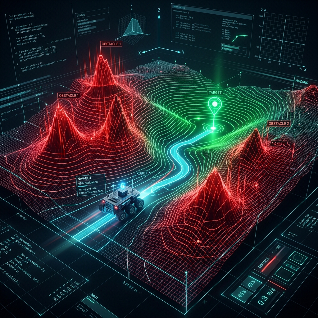
Reactive Path Planning and Collision Avoidance of Mobile Robots using Artificial Potential Fields
Section 1: Introduction to Reactive Path Planning
1.1 Paradigm of Robot Navigation: Global vs. Local Path Planning
Autonomous mobile robot navigation is fundamentally structured as a hierarchical decision-making process, traditionally partitioned into two primary layers: global path planning (deliberative planning) and local path planning (reactive planning). This division is dictated by the trade-off between the computational complexity of searching high-dimensional configuration spaces and the real-time requirements of avoiding dynamic, unmapped obstacles in physical environments.
Global path planning operates on a macro-level representation of the environment, assuming the availability of a complete, a priori map (e.g., occupancy grids, vector maps, or polygonal maps). The primary goal of a global planner is to establish a collision-free topological path from an initial robot configuration $q_{start}$ to a designated goal configuration $q_{goal}$ in the configuration space $C$. Common algorithmic methodologies include graph-search algorithms (e.g., Dijkstra's algorithm, A*) and sampling-based planners (e.g., Probabilistic Roadmaps (PRM), Rapidly-exploring Random Trees (RRT)). These methods explore the connectivity of the free configuration space $C_{free}$ to guarantee completeness or resolution completeness.
However, global path planning is computationally expensive. For example, A* search on a dense grid scales with the volume of the search space, resulting in a time complexity of:
where $V$ is the number of grid cells (vertices) and $E$ is the number of transitions between adjacent cells (edges). In a three-dimensional configuration space (e.g., representing position $x, y$ and orientation $\theta$), the number of grid cells scales cubically with resolution, making online re-computation at high frequencies (e.g., 50 Hz) infeasible. Consequently, global planners are typically executed as background processes at low frequencies (0.1 Hz to 1 Hz) or triggered only when the local environment deviates significantly from the global map.
In contrast, local path planning (or reactive path planning) operates within a limited spatial and temporal horizon, utilizing real-time sensor streams (such as LiDAR distance scans, ultrasonic rangefinder profiles, or depth camera point clouds) to generate immediate actuator commands. Local planners do not require a complete map of the environment and instead focus on the robot's immediate vicinity. The primary objective is to drive the robot towards a local target (often a waypoint on the global path) while avoiding static and dynamic obstacles that were either unmapped or not present during the global planning phase.
Reactive planning must execute at high control loop rates (typically 20 Hz to 100 Hz) to maintain control stability and safety at high velocities. Because of this speed requirement, local planners employ heuristic or analytical methods with low computational footprints, such as the Dynamic Window Approach (DWA), Velocity Obstacles (VO), Vector Field Histogram (VFH), and Artificial Potential Fields (APF). The comparative matrix below highlights the architectural differences between these two planning paradigms:
1.2 Reactive Collision Avoidance and High-Speed Real-Time Navigation Constraints
For autonomous vehicles navigating in dense or dynamic environments, reactive collision avoidance is the primary line of defense. The physical and digital parameters of the robot system impose strict constraints on the maximum safe velocity $v$ at which a robot can travel. To model these constraints, we must analyze the total system latency, braking profiles, and sensor ranges.
The total system latency $t_{delay}$ is the time elapsed between the physical detection of an obstacle and the physical onset of deceleration by the actuators. This latency is a sum of several distinct components:
where $t_{sense}$ is the sensor exposure and integration time (e.g., the time required for a LiDAR to complete a $360^\circ$ scan or for a camera to capture a frame), $t_{process}$ is the execution time of the local path planning and safety assessment algorithms, $t_{comm}$ is the communication bus latency (e.g., CAN bus propagation, Ethernet transmission delays, or ROS message serialization overhead), and $t_{act}$ is the mechanical response time of the motor drives and braking systems (e.g., the electrical time constant of the motor windings and the mechanical response of brake calipers or electromagnetic couplers).
During the interval $t_{delay}$, the robot continues to travel at its initial linear velocity $v_0$. Assuming a worst-case scenario where the robot is traveling at $v_0$ towards a stationary obstacle, the distance traveled during this reaction phase is:
Once the actuators initiate braking, the robot undergoes deceleration. Assuming a constant maximum deceleration limit $a_{max}$ (which is bounded by the motor torque capacity and the friction coefficient between the tires/tracks and the ground), the distance required to bring the robot to a complete stop is derived from basic kinematic equations:
The total stopping distance $d_{stop}$ is the sum of the reaction distance and the braking distance:
To guarantee that the robot can avoid a collision with any obstacle detected in its direction of travel, the range of the sensor system $d_{sense}$ (excluding range measurement noise and uncertainty) must be strictly greater than the stopping distance plus a safety margin $d_{safe}$:
We can rearrange this inequality as a quadratic function of the velocity $v_0$ to determine the maximum safe operating velocity $v_{max}$ of the robot:
Applying the quadratic formula to solve for the positive root of the corresponding quadratic equation:
Simplifying this expression yields:
This formula defines the dynamic operating envelope for high-speed navigation. If the sensor scan frequency drops (increasing $t_{delay}$) or the coefficient of friction decreases due to wet surface conditions (decreasing $a_{max}$), the local planner must scale down the robot's reference velocity to satisfy this safety boundary.
1.3 Robot Motion Control and the Control Loop Architecture
A key challenge in reactive path planning is translating high-level path plans or virtual force vectors into physical control signals that respect the kinematic and dynamic constraints of the robot.
Mobile robots are classified by their kinematic capabilities, which are modeled as holonomic or non-holonomic constraints. A holonomic robot (e.g., a robot equipped with omnidirectional Mecanum wheels) can translate in any direction in the 2D plane without rotating. Its configuration is defined by its position vector $q = [x, y]^T$, and its instantaneous velocity vector $\dot{q} = [\dot{x}, \dot{y}]^T$ is unconstrained. For such a robot, a virtual force vector $F$ generated by a potential field can be directly mapped to a proportional velocity command:
However, most wheeled mobile robots (e.g., differential-drive systems, unicycles, and Ackermann-steered vehicles) are subject to non-holonomic constraints. These systems are characterized by rolling-without-slipping conditions, which restrict the direction of the robot's instantaneous velocity but do not restrict its reachable configuration space.
Consider a differential-drive robot modeled using unicycle kinematics. The robot configuration is described by the state vector $q = [x, y, \theta]^T$, where $(x, y)$ represents the coordinates of the midpoint of the wheel axle in the global frame, and $\theta$ represents the heading angle relative to the global x-axis. The kinematic model of the system is given by:
where $v$ is the linear velocity and $\omega$ is the angular velocity of the robot. The non-holonomic constraint, which mathematically represents the inability of the wheels to slip sideways, is formulated as:
Because of this constraint, the robot cannot directly execute an arbitrary force vector $F = [F_x, F_y]^T$ generated by a potential field if the force has a lateral component (i.e., perpendicular to the robot's heading $\theta$). To bridge this gap, we must design a control law that translates the virtual force vector into control inputs $[v, \omega]^T$.
One common method is input-output feedback linearization. Instead of controlling the center of rotation $(x, y)$, we define a tracking point $p = [x_p, y_p]^T$ offset from the axle center by a small distance $b > 0$ along the longitudinal axis of the robot:
Differentiating this tracking point with respect to time:
Substituting the unicycle kinematics $\dot{x} = v \cos\theta$, $\dot{y} = v \sin\theta$, and $\dot{\theta} = \omega$:
The matrix $R(\theta)$ is the decoupling matrix. The determinant of this matrix is:
Since $b > 0$, the determinant is non-zero, making the decoupling matrix $R(\theta)$ invertible for all headings $\theta$. Its inverse is given by:
If we define the desired velocity of the tracking point to be equal to the virtual force vector generated by the artificial potential field, $\dot{p} = F_{net}(p) = [F_{net, x}, F_{net, y}]^T$, we can solve for the linear and angular velocities:
By expanding this matrix multiplication, we obtain the decoupled control inputs:
This feedback linearization control law provides a continuous mapping from the potential field forces directly to the wheels' velocity commands. It guarantees that the tracking point $p$ behaves exactly as a point mass subject to the virtual force field, resolving the non-holonomic constraint issue.
Section 2: Mathematical Formulation of Potential Fields
2.1 Introduction to the Artificial Potential Field (APF) Concept
The Artificial Potential Field (APF) method, originally introduced by Oussama Khatib in 1985, is a reactive path planning framework modeled on physical field phenomena, such as electrostatic, gravitational, and fluid flow fields. In this framework, the robot is modeled as a point mass moving within a configuration space $C$. The environment is populated by virtual energy potentials that exert virtual forces on the robot.
The total artificial potential field $U(q)$ experienced by a robot at configuration $q$ is defined as the superposition of two primary components: an attractive potential field $U_{att}(q)$ and a set of repulsive potential fields $U_{rep, i}(q)$ associated with each obstacle $i$ in the workspace:
where $M$ represents the total number of detected obstacles. The attractive potential field is designed to have a global minimum at the target destination configuration $q_{goal}$, acting as a gravitational basin that pulls the robot toward the goal. The repulsive potential fields are designed to generate high potential barriers surrounding the obstacles, preventing the robot from entering these regions.
The virtual force vector field $F(q)$ acting on the robot at configuration $q$ is defined as the negative gradient of the scalar potential function $U(q)$ with respect to the robot's configuration:
where:
By modeling the robot as a point mass in this conservative vector field, the robot's path is generated by following the direction of the net virtual force $F(q)$, which corresponds to the direction of steepest descent on the potential energy surface.
2.2 Rigorous Formulation of the Attractive Potential Field
The attractive potential field $U_{att}(q)$ must be a continuously differentiable ($C^1$) scalar function that monotonically increases with the Euclidean distance between the robot configuration $q$ and the goal configuration $q_{goal}$. The most common formulation is the quadratic potential:
where $\xi$ is a positive scaling gain and $d(q, q_{goal})$ is the Euclidean distance, defined in $N$-dimensional space as:
The physical interpretation of this quadratic formulation is analogous to a Hookean spring attached to the robot at one end and the goal at the other. The potential energy is proportional to the square of the displacement. Taking the negative gradient of $U_{att}(q)$, we derive the virtual attractive force:
This attractive force increases linearly with the distance from the goal. While this linear scaling provides strong convergence when the robot is near the goal, it presents a practical hazard when the robot is very far away. If $d(q, q_{goal})$ is large, the resulting virtual force can exceed the physical velocity and torque limits of the robot (actuator saturation), which can lead to unstable steering dynamics and computational windup in control systems.
To resolve this saturation issue, we can use a conical potential field when the robot is far from the goal. The conical potential grows linearly with distance rather than quadratically:
Taking the negative gradient of this conical potential yields a force of constant magnitude:
This force behaves like a constant pull of magnitude $\xi$ directed toward the goal, preventing velocity command saturation at large distances. However, the conical potential is non-differentiable at the goal ($d(q, q_{goal}) = 0$), where the unit vector direction becomes discontinuous, which can cause the robot to oscillate around the goal rather than coming to a smooth stop.
To combine the advantages of both approaches, we can construct a hybrid attractive potential field. This potential is quadratic when the robot is within a transition distance $d_{tr}$ from the goal, and switches to a conical form outside this threshold:
We can prove that this hybrid function is continuously differentiable ($C^1$ continuous) across the boundary $d(q, q_{goal}) = d_{tr}$. First, we check the continuity of the potential function itself ($C^0$ continuity) at the boundary:
Since the left and right limits are equal, the potential function is continuous at the boundary. Next, we verify the continuity of the gradient ($C^1$ continuity) by computing the gradient of both segments. For $d(q, q_{goal}) \le d_{tr}$:
For $d(q, q_{goal}) > d_{tr}$, using the chain rule:
Evaluating these gradients at the boundary $d(q, q_{goal}) = \|q - q_{goal}\| = d_{tr}$ gives:
Because the gradients match exactly at the boundary, the hybrid attractive potential is $C^1$ continuous. The corresponding force vector $F_{att}(q)$ is:
This formulation ensures that when the robot is far from the goal, it is pulled by a constant force of magnitude $\xi d_{tr}$, and as it enters the local neighborhood $d_{tr}$, the force decreases linearly, allowing the robot to settle smoothly at the goal configuration.
2.3 Rigorous Formulation of the Repulsive Potential Field
The repulsive potential field $U_{rep}(q)$ is designed to prevent the robot from colliding with obstacles. To ensure the robot is only affected by obstacles in its immediate vicinity, the repulsive potential is active only within a local influence zone defined by a threshold distance $d_0$. The classical formulation of the repulsive potential is:
where $\eta$ is a positive repulsive gain, $d(q, q_{obs})$ represents the shortest Euclidean distance from the robot configuration $q$ to the surface of the obstacle, and $d_0$ is the sensor-limited range of influence.
The physical reasoning behind this formulation is as follows:
- Boundary Smoothness: At the boundary of the influence zone ($d(q, q_{obs}) = d_0$), the potential is exactly zero: $U_{rep}(q) = \frac{1}{2} \eta \left( \frac{1}{d_0} - \frac{1}{d_0} \right)^2 = 0$. This ensures that the potential transitions smoothly to zero at the boundary, avoiding discontinuous jumps.
- Asymptote at Collision: As the robot approaches the obstacle surface ($d(q, q_{obs}) \to 0$), the term $\frac{1}{d(q, q_{obs})} \to \infty$. The potential energy grows asymptotically to infinity, creating an impassable barrier that prevents the robot from contacting the obstacle.
To derive the virtual repulsive force $F_{rep}(q) = -\nabla U_{rep}(q)$ for a robot within the active zone ($d(q, q_{obs}) \le d_0$), we apply the chain rule of calculus. Let $d_{obs}(q) = d(q, q_{obs}) = \|q - q_{obs}\|$. The gradient of this distance function is:
Now, we define $u(q) = \frac{1}{d_{obs}(q)} - \frac{1}{d_0}$, so that $U_{rep}(q) = \frac{1}{2} \eta u(q)^2$. Differentiating $U_{rep}(q)$ with respect to $q$:
The gradient of $u(q)$ is:
Substituting $\nabla u(q)$ back into the expression for $\nabla U_{rep}(q)$:
The repulsive force $F_{rep}(q)$ is the negative gradient of the potential, $F_{rep}(q) = -\nabla U_{rep}(q)$:
We can express the force in terms of the unit direction vector pointing from the obstacle to the robot, defined as:
Substituting $\hat{u}_{obs}$ into the force equation:
This formula shows that the repulsive force points directly away from the obstacle along the line of shortest distance, and its magnitude scales inversely with the cube of the distance as the robot gets closer ($d(q, q_{obs}) \to 0$).
2.4 Gradient Operations and Full Component Resolution
To implement this algorithm in real-time control software, the force vectors must be resolved into their scalar components along each coordinate axis. Below, we derive these component equations for both two-dimensional (2D) and three-dimensional (3D) configuration spaces.
2.4.1 Two-Dimensional Component Resolution
Let the robot position in the plane be $q = [x, y]^T$, the goal configuration be $q_{goal} = [x_g, y_g]^T$, and the obstacle position be $q_{obs} = [x_o, y_o]^T$.
The Euclidean distances in 2D are:
Attractive Force (Quadratic Regime):
The quadratic attractive potential in 2D is:
Taking the partial derivatives:
The attractive force components are:
Attractive Force (Conical Regime):
The conical attractive potential in 2D is:
Taking the partial derivatives:
The attractive force components in the conical regime are:
Repulsive Force (Active Zone):
Let $d_{obs} = \sqrt{(x - x_o)^2 + (y - y_o)^2} \le d_0$. The repulsive potential is:
Differentiating with respect to $x$ using the chain rule:
Similarly, differentiating with respect to $y$:
Because the force components are the negative partial derivatives ($F_x = -\frac{\partial U}{\partial x}$, $F_y = -\frac{\partial U}{\partial y}$), we have:
The net force vector in 2D is the vector sum of these components:
2.4.2 Three-Dimensional Component Resolution
Let the robot position in 3D space be $q = [x, y, z]^T$, the goal configuration be $q_{goal} = [x_g, y_g, z_g]^T$, and the obstacle position be $q_{obs} = [x_o, y_o, z_o]^T$.
The Euclidean distances in 3D are:
Attractive Force (Quadratic Regime):
Attractive Force (Conical Regime):
Repulsive Force (Active Zone):
For $d(q, q_{obs}) \le d_0$:
The net force vector in 3D is:
2.4.3 Mathematical Proof of Conservative Field Properties
A key mathematical property of the artificial potential field approach is that the resulting force field $F(q)$ is conservative. In physics, a vector field is conservative if it is the gradient of a scalar potential function. A critical consequence of this property is that the curl of the force field is zero everywhere in the workspace (excluding the singularities at the obstacle boundaries):
We can prove this property in a 3D configuration space. Let the virtual force field be $F(q) = [F_x, F_y, F_z]^T = -\nabla U(q) = \left[ -\frac{\partial U}{\partial x}, -\frac{\partial U}{\partial y}, -\frac{\partial U}{\partial z} \right]^T$. The curl operator in Cartesian coordinates is defined as the determinant of the formal matrix:
Expanding this determinant yields:
Substitute the partial derivatives of the scalar potential function $U(q)$ into the first component:
According to Clairaut's Theorem (also known as the Schwarz theorem on mixed partial derivatives), if a scalar function $U(q)$ is twice continuously differentiable ($C^2$), then its mixed partial derivatives are independent of the order of differentiation:
Substituting this equivalence back into the component equation:
Applying the same substitution to the remaining components:
Thus, all components of the curl vector are zero:
This mathematical proof confirms that the force field is conservative. In practice, this means we can use energy-like Lyapunov stability proofs to analyze the robot's motion. The total potential function $U(q)$ can serve as a candidate Lyapunov function. If we choose a control law that moves the robot in the direction of steepest descent, we can guarantee that the robot's energy decreases continuously until it reaches a local or global minimum.
Section 3: The Local Minima Problem and Mathematical Fixes
3.1 Mathematical Analysis of the Local Minima Problem
The primary limitation of the Artificial Potential Field method is the existence of local minima. A local minimum is a configuration $q_{lm}$ where the net virtual force acting on the robot is zero, but which does not correspond to the target configuration:
A configuration where $\nabla U(q) = 0$ is a critical point. To classify a critical point, we compute the Hessian matrix $H(q)$ of the potential function. The Hessian is the symmetric matrix of second-order partial derivatives:
At any critical point $q_c$ (where $\nabla U(q_c) = 0$), we can classify its stability by analyzing the eigenvalues $\lambda_i$ of the Hessian matrix $H(q_c)$:
- Local Minimum: The Hessian is positive definite (all eigenvalues $\lambda_i > 0$). In this case, any displacement away from $q_c$ increases the potential energy. The surrounding force field points back toward $q_c$, trapping the robot at this point.
- Local Maximum: The Hessian is negative definite (all eigenvalues $\lambda_i < 0$). Displacement away from $q_c$ decreases the potential energy. The force field points away from $q_c$, repelling the robot.
- Saddle Point: The Hessian is indefinite, having both positive and negative eigenvalues ($\lambda_{min} < 0 < \lambda_{max}$). In this case, some directions of displacement increase the potential energy, while others decrease it. While saddle points are unstable, they can slow down convergence because the gradient forces near them are very small.
To illustrate the creation of a local minimum, we analyze a collinear environment. Consider a robot at $q = [x, y]^T$, a goal at the origin $q_{goal} = [0, 0]^T$, and a single point obstacle placed at $q_{obs} = [d_{obs}, 0]^T$ along the positive x-axis, where $d_{obs} > 0$. We assume the robot is positioned further down the positive x-axis at $q = [x, 0]^T$, where $x > d_{obs}$.
The attractive force (using the quadratic formulation) is directed along the x-axis toward the origin:
Because the robot is at $x > d_{obs}$, the distance to the obstacle is $d(q, q_{obs}) = x - d_{obs}$. The repulsive force (assuming $d(q, q_{obs}) \le d_0$) points in the positive x-direction, away from the obstacle:
The net force acting on the robot along the x-axis is:
We can prove the existence of a local minimum along the x-axis on the interval $x \in (d_{obs}, d_{obs} + d_0)$ using the Intermediate Value Theorem.
First, we evaluate the limit of the net force as the robot approaches the obstacle from the right:
Second, we evaluate the net force at the boundary of the obstacle's influence zone, $x = d_{obs} + d_0$:
Since $F_{net, x}(x)$ is continuous on the open interval $(d_{obs}, \infty)$, and it changes sign from positive to negative on the sub-interval $[d_{obs}, d_{obs} + d_0]$, the Intermediate Value Theorem guarantees that there exists at least one point $x^* \in (d_{obs}, d_{obs} + d_0)$ such that:
At this point $x^*$, the attractive force pulling the robot toward the origin is balanced by the repulsive force pushing it away from the obstacle. To determine the stability of this equilibrium, we calculate the derivative of the net force with respect to $x$ at this point:
Factoring out terms to analyze the sign:
For any point within the influence zone, $x - d_{obs} < d_0 \implies \frac{2(x - d_{obs})}{d_0} < 2$. Thus, the term inside the parenthesis is strictly positive:
Since $\xi > 0$, $\eta > 0$, and $(x - d_{obs})^4 > 0$, the entire expression for the derivative is strictly negative:
The Hessian component of the potential field is the negative derivative of the net force:
Because this second-order derivative is positive, $x^*$ is a local minimum along the x-axis. If the robot is displaced slightly to the right ($x > x^*$), the net force becomes negative, pulling it back to the left. If it is displaced to the left ($x < x^*$), the net force becomes positive, pushing it back to the right. The robot is trapped at this local minimum, unable to reach the goal.
3.2 The GNRON (Goal Non-Reachable with Obstacles Nearby) Problem
A specific case of the local minima problem occurs when an obstacle is located very close to the goal. Specifically, if the goal configuration lies within the influence zone of an obstacle:
This scenario is known as the Goal Non-Reachable with Obstacles Nearby (GNRON) problem. As the robot approaches its target, the attractive potential decreases, and the attractive force vanishes at the goal:
However, because the goal lies within the obstacle's influence zone, the repulsive force does not go to zero. Instead, it converges to a non-zero constant vector pointing away from the obstacle:
Since $d(q_{goal}, q_{obs}) < d_0$, the coefficient is positive:
Consequently, the net virtual force at the goal is non-zero:
Because the net force at the goal is non-zero, the goal configuration is no longer an equilibrium point of the system. The robot cannot stabilize at the goal. Instead, it will settle at a shifted equilibrium point $q_{eq} \neq q_{goal}$ where the attractive and repulsive forces balance each other:
This shifted equilibrium point lies along the line connecting the obstacle to the goal, but is offset away from the obstacle. As a result, the robot will stop prematurely before reaching the goal, or it will oscillate around the target. This behavior is undesirable for applications requiring high precision, such as docking or target manipulation.
3.3 Mathematical Modifications to Resolve GNRON
To resolve the GNRON problem, we can modify the repulsive potential function by multiplying it by a term containing the distance to the goal. The modified repulsive potential function is defined as:
where $n$ is a positive integer parameter (typically $n = 2$). The addition of the goal distance term $d(q, q_{goal})^n$ ensures that the repulsive potential drops to zero at the goal configuration, even if the goal is close to an obstacle.
3.3.1 Derivation of the Modified Gradient
For $d_{obs}(q) \le d_0$, let $d_{obs}(q) = d(q, q_{obs}) = \|q - q_{obs}\|$ and $d_{goal}(q) = d(q, q_{goal}) = \|q - q_{goal}\|$. We compute the gradient of the modified repulsive potential using the product rule:
We evaluate the gradients of the individual terms:
Substituting these back into the expression for $\nabla U_{rep}(q)$:
Simplifying this expression:
The modified repulsive force $F_{rep}(q) = -\nabla U_{rep}(q)$ is the sum of two component forces:
where:
The physical and geometric roles of these two forces are:
- $F_{rep1}(q)$ (Repulsive Direction): This force points in the direction of the vector $(q - q_{obs})$, pushing the robot away from the obstacle. However, its magnitude is scaled by the distance-to-goal term $d(q, q_{goal})^n$. As the robot approaches the goal ($d(q, q_{goal}) \to 0$), this repulsive term is scaled down and vanishes. This allows the robot to approach obstacles near the goal.
- $F_{rep2}(q)$ (Attractive Direction): This force points in the direction of the vector $-(q - q_{goal}) = (q_{goal} - q)$, which pulls the robot toward the goal. The magnitude of this force is proportional to the distance-to-obstacle term $\left( \frac{1}{d(q, q_{obs})} - \frac{1}{d_0} \right)^2$. This acts as a virtual attractive force that pulls the robot toward the goal when it is near an obstacle, helping it overcome the repulsive barrier.
3.3.2 Proof of Goal Convergence
We can prove that the goal configuration $q_{goal}$ is a stable equilibrium point under this modified potential field. We assume the parameter $n = 2$ and that the obstacle is not located exactly at the goal, i.e., $d(q_{goal}, q_{obs}) > 0$.
First, we verify that the goal is a critical point ($\nabla U(q_{goal}) = 0$). Evaluating the first force component $F_{rep1}(q)$ at $q = q_{goal}$:
Next, we evaluate the second force component $F_{rep2}(q)$ for $n = 2$ at $q = q_{goal}$:
Thus, the modified repulsive force vanishes at the goal:
Since the attractive force also vanishes at the goal ($\nabla U_{att}(q_{goal}) = 0$), the net potential gradient at the goal is zero:
This confirms that the goal configuration is a critical point.
To verify that the goal is a stable local minimum, we calculate the Hessian matrix of the total potential field at $q = q_{goal}$. The total potential is:
For a quadratic attractive potential, the Hessian is a constant diagonal matrix:
where $I$ is the identity matrix.
For the modified repulsive potential (with $n = 2$), we define the scalar function:
This allows us to write the modified repulsive potential as:
We compute the gradient of this product:
Next, we calculate the Jacobian of this gradient to find the Hessian matrix $\nabla^2 U_{rep}(q)$:
Using the product and tensor rules:
At the goal configuration, $q = q_{goal}$, the vector difference is zero: $(q - q_{goal}) = 0$. Consequently, the terms involving $(q - q_{goal})$ and $\|q - q_{goal}\|^2$ vanish:
Substituting the definition of $g(q)$ back in:
The total Hessian matrix at the goal configuration is the sum of the attractive and repulsive Hessians:
Since $\xi > 0$ and the squared term is non-negative, the scalar coefficient is strictly positive:
Because the scalar coefficient is positive, all eigenvalues of $H(q_{goal})$ are strictly positive:
This proof confirms that the Hessian matrix $H(q_{goal})$ is positive definite. Consequently, the goal configuration $q_{goal}$ is a strict local minimum of the total potential field, resolving the GNRON problem. Even if an obstacle is placed very close to the goal, the robot will converge to the target location.
3.3.3 Component Resolution of the Modified Repulsive Force
We resolve this modified repulsive force into coordinate components in 2D and 3D.
2D C-space Component Resolution:
For $n = 2$, let $d_{obs} = \sqrt{(x - x_o)^2 + (y - y_o)^2}$ and $d_{goal} = \sqrt{(x - x_g)^2 + (y - y_g)^2}$. The components of the modified repulsive force $F_{rep}(q) = [F_{rep, x}, F_{rep, y}]^T$ are:
3D C-space Component Resolution:
Let $d_{obs} = \sqrt{(x - x_o)^2 + (y - y_o)^2 + (z - z_o)^2}$ and $d_{goal} = \sqrt{(x - x_g)^2 + (y - y_g)^2 + (z - z_g)^2}$. The components of the modified repulsive force $F_{rep}(q) = [F_{rep, x}, F_{rep, y}, F_{rep, z}]^T$ are:
3.3.4 Review of Alternative Solutions
While the modified repulsive potential resolves the GNRON problem, it does not eliminate all local minima in complex environments, such as U-shaped obstacles or symmetric configurations. Researchers have developed several alternative methodologies to address these cases:
- Navigation Functions: Developed by Rimon and Koditschek, navigation functions are specialized potential functions that are guaranteed to have only one minimum (at the goal) on sphere worlds. All other critical points are designed to be unstable saddle points, preventing the robot from getting trapped.
- Harmonic Potential Fields: These fields are designed by solving Laplace's equation $\nabla^2 U = 0$ with Dirichlet boundary conditions ($U = 0$ at the goal, $U = 1$ on obstacles). According to the maximum principle of harmonic functions, these fields cannot contain local minima in the interior of the domain, eliminating the local minima problem entirely. However, they are computationally expensive to calculate in real-time.
- Virtual Obstacles and Escaping Algorithms: If a local minimum is detected (e.g., when the net force is near zero but the robot has not reached the goal, $\|F_{net}\| < \epsilon$), the robot can apply a temporary virtual force (e.g., perpendicular to the line of centers) or place a temporary virtual obstacle at its current coordinates. This perturbs the potential field, pushing the robot out of the trap.
- Hybrid Path Planners (APF-RRT): In this approach, the artificial potential field method is combined with a sampling-based planner. The robot uses the APF method for fast, reactive navigation. If it detects a local minimum, the system activates a local RRT planner to find a path segment out of the trap, returning control to the APF planner once the barrier is cleared.
Figure 1: 2D Path Planning in Artificial Potential Fields
A real-time simulation showing the mobile robot planning its path from the Start point to the Goal. The local coordinate frame (x_r, y_r) rotates dynamically as the robot adjusts its heading, and the lidar sweeps for obstacle boundaries.
Figure 2: 3D Potential Field Landscape Mesh
A 3D-like isometric mesh representing the artificial potential landscape. The obstacles create repulsive peaks (high potential), while the goal forms an attractive valley (global minimum). The robot (represented as a rolling ball) navigates the slopes via gradient descent.
Figure 3: Interactive Vector Field Dashboard
An interactive dashboard showing the vector field (net force directions). Drag the green Goal or red Obstacle to dynamically re-calculate the vector fields. The blue mobile robot automatically adjusts its trajectory in real-time.
Figure 4: Geometric Force Resolution Diagram
A geometric breakdown of the potential field forces acting on a mobile robot at position q. The net force F_net is the vector sum of the attractive force F_att (towards the goal) and the repulsive force F_rep (pointing away from the obstacle within its influence circle d_0).
4. Detailed Numerical Worked Example
In order to bridge the gap between theoretical formulation and practical implementation, this section provides a comprehensive, step-by-step numerical worked example. We calculate the attractive, repulsive, and net force vectors for a mobile robot operating in a continuous two-dimensional space. By following the algebraic evaluations, coordinate transformations, and gradient operations, the reader will gain a concrete understanding of how potential fields govern robot kinematics in real time. We then execute a first-order Euler integration step to determine the robot's updated position vector.
4.1. Setup of the Kinematic Navigation Environment
Consider a point-mass holonomic mobile robot located at the instantaneous coordinate vector $q \in \mathbb{R}^2$. The workspace is populated by a single target goal and one circular obstacle. The coordinates, scaling parameters, and system gains are defined below:
- Robot position: $q = \begin{bmatrix} 2.0 \\ 3.0 \end{bmatrix}$ (meters)
- Goal position: $q_{\text{goal}} = \begin{bmatrix} 10.0 \\ 10.0 \end{bmatrix}$ (meters)
- Obstacle center position: $q_{\text{obs}} = \begin{bmatrix} 5.0 \\ 6.0 \end{bmatrix}$ (meters)
- Obstacle radius: $R = 1.0$ (meter)
- Obstacle influence threshold: $d_0 = 3.0$ (meters)
- Attractive potential gain: $k_a = 1.0$ (dimensionless or $\text{s}^{-2}$ mapping to force)
- Repulsive potential gain: $k_r = 15.0$ ($\text{N}\cdot\text{m}^2$)
- Integration step time: $dt = 0.1$ (seconds)
The robot is governed by first-order kinematic equations, implying that its velocity vector $\dot{q}(t)$ is directly proportional to the applied virtual net force vector $F_{\text{net}}(q(t))$. Assuming a virtual damping coefficient $\gamma = 1.0 \text{ N}\cdot\text{s/m}$, the state transition equation is simplified as:
This direct mapping means the robot's velocity vector (in meters per second) is numerically identical to the net force vector (in Newtons) generated by the potential field gradients.
4.2. Analytical Calculation of the Attractive Force Vector
The attractive potential field is modeled as a quadratic function of the Euclidean distance to the goal, ensuring a linear growth of the attractive force as the robot moves further away. The attractive potential $U_{\text{att}}(q)$ and its gradient-derived attractive force $F_{\text{att}}(q)$ are formulated as:
To compute $F_{\text{att}}(q)$ at the robot's current coordinates, we first compute the displacement vector:
The Euclidean distance from the robot to the goal is calculated as:
Substituting $k_a = 1.0$ into the force expression yields:
4.3. Assessment of Repulsive Potential (Scenario A: $d_0 = 3.0$ m)
The shortest Euclidean distance from the robot center to the surface boundary of the circular obstacle is denoted as $\rho(q)$, calculated as:
First, we find the displacement vector from the obstacle center to the robot:
The distance from the robot to the obstacle center is:
Subtracting the obstacle radius $R = 1.0$ m yields the surface-to-surface distance:
The repulsive potential function $U_{\text{rep}}(q)$ is activated only when the robot's surface distance falls below the threshold $d_0$. The general piecewise formulation is:
In Scenario A, the obstacle influence range is set to $d_0 = 3.0$ m. Comparing the surface distance to this limit:
Since the robot is outside the obstacle's zone of influence, the repulsive potential and its gradient are zero:
The net force acting on the robot is:
Applying the first-order Euler integration formula to update the robot's coordinates:
Thus, under the parameters of Scenario A, the robot moves directly toward the goal, updating its coordinates to $(2.8, 3.7)$ meters.
4.4. Gradient Derivation & Vector Arithmetic (Scenario B: Active Avoidance with $d_0 = 5.0$ m)
To demonstrate the vector math and gradient operations when the repulsive force is active, we analyze Scenario B. In this scenario, we extend the obstacle's influence limit to $d_0 = 5.0$ m. Since the surface distance is $\rho(q) = 3.24264 \text{ m} \le d_0 = 5.0 \text{ m}$, the repulsive potential is active.
First, we find the gradient of the surface distance function $\nabla \rho(q)$ using the chain rule:
This unit vector points from the center of the obstacle toward the robot position:
Now we calculate the gradient of the repulsive potential $U_{\text{rep}}(q)$. Applying the chain rule to the potential function:
The repulsive force $F_{\text{rep}}(q)$ is the negative gradient of the potential field:
We evaluate the scalar components of the force equation:
Multiplying these terms together with the repulsive gain $k_r = 15.0$ and the direction vector:
This repulsive force vector acts to push the robot away from the obstacle (in the southwest direction).
4.5. Calculation of the Net Force Vector and Numerical Integration
The net force acting on the robot is the vector sum of the attractive and repulsive forces:
Using the first-order Euler integration formula with $dt = 0.1$ s, we calculate the robot's updated position:
Comparing the two scenarios shows the physical effect of the active obstacle. In Scenario A (no obstacle influence), the robot moved to $(2.8, 3.7)$ m. In Scenario B, the active repulsive force reduced the displacement in both axes by approximately $1.09$ cm, resulting in a position of $(2.7891, 3.6891)$ m. This reduction in step size and change in direction shows the robot slowing down and starting to steer around the obstacle's boundary.
6. Advanced Potential Field Variations & Extensions
While the classical Artificial Potential Field method is computationally simple and runs in real time, it has two major limitations: it is prone to local minima, and it struggles to handle moving obstacles. A local minimum occurs when the attractive and repulsive forces cancel each other out ($F_{\text{net}}(q) = 0$) at a position other than the goal ($q \neq q_{\text{goal}}$), trapping the robot. To address these issues, roboticists have developed advanced potential field variations.
6.1. Harmonic Potential Fields and Laplace Panel Methods
Harmonic Potential Fields (HPFs) eliminate local minima by using harmonic functions, which are solutions to Laplace's differential equation. A real-valued function $U(q)$ is harmonic in a domain $\Omega \subset \mathbb{R}^n$ if it satisfies Laplace's equation:
Harmonic functions satisfy the Maximum Principle: a harmonic function defined on a closed, bounded domain $\Omega$ cannot reach a local maximum or minimum in the interior of that domain; all local extrema must lie on the boundary $\partial \Omega$. By setting the goal point as a global sink (minimum potential) and the obstacle boundaries as sources (maximum potential), the potential field is guaranteed to have no local minima in the robot's free space. This ensures that following the negative gradient path always leads to the goal.
To resolve Laplace's equation in complex environments in real-time, designers borrow numerical methods from fluid dynamics, particularly panel methods. In a panel method, the boundaries of obstacles are represented as a set of flat line segments (in 2D) or planar triangles (in 3D), called panels. Each panel $j$ is treated as a continuous distribution of virtual fluid sources or sinks with a strength density $\lambda_j$. The potential field $U(q)$ at any point $q$ in the workspace is the sum of the potential from the goal (a point sink) and the potentials from all boundary panels:
Here, $s$ represents coordinates along the surface of panel $j$, and $M$ is the total number of panels. We determine the source strengths $\lambda_j$ by enforcing boundary conditions. The two main boundary condition types are:
- Dirichlet Boundary Condition: The potential is set to a constant high value on the obstacle boundaries ($U(q) = c_{\text{max}}$ for $q \in \partial\Omega_{\text{obs}}$). This creates a high potential barrier.
- Neumann Boundary Condition: The normal derivative of the potential is set to zero on the obstacle boundaries ($\nabla U(q) \cdot \hat{n} = 0$ for $q \in \partial\Omega_{\text{obs}}$, where $\hat{n}$ is the unit normal vector to the boundary). This ensures the robot's path flows smoothly around obstacles, similar to fluid flowing around a solid object.
Using the Neumann condition, we construct a linear system $A \lambda = B$, where $A \in \mathbb{R}^{M \times M}$ is the influence coefficient matrix representing the geometric relationships between the panels, $\lambda = [\lambda_1, \dots, \lambda_M]^T$ is the vector of source strengths, and $B \in \mathbb{R}^M$ represents the influence of the goal sink on each panel's midpoint. Solving this system gives the panel strengths $\lambda$. Once $\lambda$ is known, the robot's velocity command is computed directly from the gradient:
This approach ensures a smooth path to the goal without local minima. However, panel methods are computationally expensive. Setting up and solving the linear equation system requires $O(M^3)$ operations using direct methods, or $O(M^2)$ using iterative solvers, where $M$ is the number of boundary panels. For complex, dynamic environments, this computational cost can limit real-time performance on resource-constrained microcontrollers.
6.2. Evolutionary Potential Fields for Adaptive Tuning
Evolutionary Potential Fields (EPFs) combine meta-heuristic optimization algorithms—such as Genetic Algorithms (GA) or Particle Swarm Optimization (PSO)—with potential fields. EPFs are used for two primary tasks: tuning potential field parameters in real-time, and generating temporary sub-goals (waypoints) to escape local minima when the robot gets stuck.
In complex environments, fixed gains ($k_a, k_r, d_0$) can cause issues. If $k_r$ is too high, the robot may oscillate near obstacles; if it is too low, the robot may collide with them. EPFs solve this by dynamically tuning these parameters based on the local environment. A swarm of virtual candidate configurations (particles or chromosomes) searches for the best parameter values by minimizing a cost function. The optimization objective function $J$ is defined as:
where $w_1, w_2, w_3$ are weighting coefficients, $\dot{q}_{\text{ref}}$ is the desired target velocity, and $d_{\text{safe}}$ is the minimum safety clearance. This cost function balances path smoothness, reference velocity tracking, and collision avoidance.
If a local minimum is detected—indicated by the robot's velocity dropping below a threshold while far from the goal ($\|\dot{q}\| < \epsilon$ and $\|q - q_{\text{goal}}\|_2 > D_{\text{threshold}}$)—the EPF system generates temporary sub-goals. The evolutionary algorithm runs a fast optimization loop to find a coordinate $q_{\text{sub}}$ in the robot's local free space. The ideal sub-goal is close to the robot, maintains a safe distance from obstacles, and has a clear line of sight to the final goal. The optimization problem is formulated as:
Once the algorithm finds the optimal $q_{\text{sub}}^*$, the robot temporary changes its attractive force target from the final goal to this sub-goal. This pulls the robot out of the local minimum and around the obstacle. Once the robot passes the obstacle and a clear path to the final goal is restored, the attractive target reverts to $q_{\text{goal}}$. While effective, the main challenge of EPFs is their high computational demand. Running evolutionary optimization loops online requires significant processing power, which can limit their use on low-power microcontrollers.
6.3. Velocity-Dependent Potential Fields for Dynamic Environments
Static potential fields do not account for the velocity of moving obstacles, which can lead to collisions or overly conservative path planning in dynamic environments. Velocity-Dependent Potential Fields (VDPFs) address this by incorporating the relative velocity between the robot and obstacles into the potential function.
Let $v = \dot{q}$ be the robot's velocity vector and $v_{\text{obs}}$ be the velocity vector of a moving obstacle. The relative velocity vector is defined as $v_{\text{rel}} = v - v_{\text{obs}}$. VDPF uses this relative velocity to adjust the repulsive potential: if the obstacle is moving away from the robot, the repulsive force is reduced; if they are approaching each other, the repulsive force is increased. The potential function is modeled as:
Here, $\theta$ is the angle between the relative velocity vector $v_{\text{rel}}$ and the relative position vector $r_{\text{obs}} = q_{\text{obs}} - q$. The condition $\cos\theta > 0$ means the robot and obstacle are moving toward each other:
The term $d_0(v_{\text{rel}})$ dynamically scales the obstacle's influence range based on the relative velocity:
where $d_{\text{min}}$ is the static safety clearance and $\tau$ is a time-to-collision factor. The scaling function $f(v_{\text{rel}}, \theta)$ is designed to increase the repulsive force when the relative velocity is high and the collision angle is direct:
The gradient of this potential function with respect to the robot's position $q$ determines the repulsive force vector. Because the potential depends on both position and velocity, the force expression includes terms for both spatial and velocity variations:
This formula adjusts the repulsive force based on the dynamics of the situation. If a moving obstacle crosses the robot's path, the potential field stretches in the direction of the obstacle's motion. This causes the robot to steer behind the moving obstacle rather than trying to cross in front of it. While VDPFs improve safety in dynamic environments, they require accurate velocity measurements for both the robot and nearby obstacles, which can be challenging to obtain using on-board sensors.
6.4. Comparative Analysis of Potential Field Methodologies
Each potential field variant offers a different balance of computational complexity, safety, and path quality. The table below summarizes and compares the key characteristics of these methodologies.
7. Practical Hardware Implementation, Sensor Constraints, & Case Studies
Deploying Artificial Potential Field algorithms on physical robots introduces challenges not captured in simulation. Real-world systems must handle sensor noise, limited computational resources, actuator saturation, and safety regulations. This section discusses these practical challenges and explains how to address them in industrial mobile platforms.
7.1. Sensor Noise, Uncertainty, and Gradient Propagation
Physical robots use sensors like LiDAR, depth cameras, and ultrasonic sensors to detect obstacles. Every sensor has measurement noise and specific limitations:
- LiDAR Sensors: LiDARs provide accurate distance measurements but can experience noise from beam divergence, multipath reflections, or when detecting reflective or glass surfaces.
- Ultrasonic Sensors: Ultrasonic sensors are low-cost but have a wide beam angle (typically $15^\circ$ to $30^\circ$), resulting in poor angular resolution. They are also prone to specular reflections, where the signal bounces off a wall at an angle and fails to return to the sensor.
In a potential field algorithm, sensor readings are used directly to calculate distance gradients. Noise in these measurements can be amplified during gradient calculations. For example, if a LiDAR sensor detects a wall with random measurement noise $\eta \sim \mathcal{N}(0, \sigma^2)$, the calculated distance varies between samples. The gradient of the repulsive force is proportional to the inverse square of the distance ($\nabla U_{\text{rep}} \propto \frac{1}{\rho^2(q)}$). If the robot is close to an obstacle (small $\rho$), even small variations in the measured distance can cause large fluctuations in the calculated repulsive force:
This noise propagation causes high-frequency oscillations in the calculated force vector. If sent directly to the motors, these oscillations cause the robot to jitter, which increases actuator wear and wastes energy.
To prevent this, robots use filtering and estimation techniques. Instead of calculating forces directly from raw sensor data, they update a probabilistic 2D occupancy grid map (e.g., using log-odds mapping). The potential field is then calculated using the filtered occupancy values. Alternatively, raw force vectors can be smoothed using a low-pass filter:
where $\beta \in [0.8, 0.95]$ is a smoothing factor. This filter reduces high-frequency jitter but introduces a small time delay in the robot's response, which must be accounted for during high-speed navigation.
7.2. Embedded Microcontroller Implementation & Numerical Optimizations
Industrial AMRs use low-power embedded microcontrollers (such as ARM Cortex-M4 or M7 series) to run control loops at frequencies between 50 Hz and 200 Hz. These processors have limited memory and processing power, making floating-point operations like divisions, square roots, and trigonometric functions computationally expensive.
To run potential field algorithms efficiently on this hardware, developers use several numerical optimization techniques:
- Avoiding Square Roots: Calculating the Euclidean distance $\|q - q_{\text{obs}}\|_2$ requires a square root operation. We can avoid this during initial distance checks by comparing the squared distance directly with the squared influence range ($d^2 \le d_0^2$):
$$\Delta x^2 + \Delta y^2 \le d_0^2$$This check filters out distant obstacles using only basic arithmetic.
- Fast Inverse Square Root: When the distance and direction vector must be calculated, we can use the fast inverse square root algorithm (originally from Quake III):
$$y = \frac{1}{\sqrt{x}}$$This algorithm calculates the inverse square root using integer manipulation and a single iteration of Newton's method, which is much faster than standard division and square root operations.
- Lookup Tables: For complex, non-linear potential functions, we can pre-calculate the values and store them in lookup tables in the microcontroller's flash memory. During operation, the controller retrieves these values using bilinear interpolation, reducing the processor load.
7.3. Actuator Saturation & Non-Holonomic Kinematic Constraints
Theoretical models often assume that a robot is holonomic (can move in any direction instantly) and has unlimited motor torque. Real mobile robots, however, are typically non-holonomic (such as differential drive or Ackermann steering layouts) and have physical limits on motor speed and torque.
For a differential drive robot, the wheels cannot move sideways. The robot's motion is defined by its linear velocity $v$ and angular velocity $\omega$. The net force vector $F_{\text{net}} = [F_x, F_y]^T$ must be converted into these velocity commands. A common approach is to align the robot's heading with the force direction and scale the linear velocity based on the force magnitude:
where $K_v, K_\omega$ are control gains. We must then limit these commands to stay within the physical capabilities of the motors:
Limiting velocity commands in this way can cause the robot to deviate from the planned potential field path. For example, if the calculated force requires a sharp turn at high speed, actuator saturation will limit the turning rate, causing the robot to follow a wider arc. If this latency is not accounted for, the robot could collide with obstacles. To address this, we can integrate the potential field with a local window optimizer like the Dynamic Window Approach (DWA). DWA evaluates candidate velocity pairs ($v, \omega$) within the robot's physical acceleration limits and selects the pair that best aligns with the direction of the potential field force.
7.4. Industrial Safety Standards & Safety PLC Overrides
In industrial environments, Automated Guided Vehicles (AGVs) and Autonomous Mobile Robots (AMRs) must comply with strict safety standards, such as ISO 3691-4 and ANSI/RIA R15.08. These standards require mobile robots to have redundant, certified safety systems that operate independently of the main navigation software.
Because potential fields run on standard operating systems (like Linux with ROS) and rely on non-safety-rated sensors, they cannot be used as the primary safety mechanism. Instead, industrial AMRs use a dual-channel architecture:
- Control Layer (Non-Safety): A standard processor runs the potential field algorithm to plan smooth, efficient paths and avoid obstacles reactively.
- Safety Layer (Safety-Rated): A safety-certified PLC (e.g., Siemens Sirius or SICK Flexi Soft) monitors safety-rated laser scanners. The safety PLC defines protective zones around the robot:
- Warning Fields: If an obstacle enters this zone, the safety PLC overrides the navigation commands to slow the robot down.
- Stop Fields: If an obstacle enters this closer zone, the safety PLC cuts power to the motor actuators and engages mechanical brakes, bringing the robot to a stop.
The diagram below illustrates this hardware architecture, showing the separation between the navigation system and the safety override loop:
In this setup, the potential field handles smooth navigation, steering the robot away from obstacles before they reach the safety zones. If the potential field fails—for example, due to a software crash or an obstacle appearing suddenly—the safety PLC intervenes to prevent a collision.
7.5. Industrial Case Studies: AMRs in Warehouses and Manufacturing
Analyzing real-world applications highlights where APF algorithms are effective and where they require modifications:
Case Study 1: Logistics AMRs in Dynamic Sorting Centers
In a large e-commerce sorting center, a fleet of 200 AMRs moves bins between sorting stations. The environment is highly dynamic, with multiple robots crossing paths constantly.
Implementation: The robots use a modified APF combined with Velocity-Dependent Potential Fields. Each robot broadcasts its position and velocity to nearby robots over Wi-Fi.
Outcome: The VDPF algorithm allows robots to adjust their paths smoothly when crossing, avoiding collisions without stopping. However, in narrow corridors, the combined repulsive forces from opposing robots occasionally created local minima, causing robots to freeze. To resolve this, developers added an evolutionary coordinator that temporarily assigns one-way directions to specific corridors.
Case Study 2: AGVs in Automotive Assembly Lines
An automotive assembly line uses heavy AGVs to transport car chassis between assembly stations along fixed paths.
Implementation: The AGVs use a highly structured potential field. The desired path is modeled as a deep potential valley (attractive force toward the path center line), and factory structures are modeled as high potential walls.
Outcome: This approach keeps the AGVs centered on their paths while allowing them to steer slightly around minor floor debris. If an obstacle blocks the path completely, the AGV stops safely rather than steering off-path into assembly areas, meeting factory safety requirements.
These case studies show that while potential fields are useful for real-time obstacle avoidance, they must be integrated with safety systems and higher-level path planners to work reliably in industrial environments.