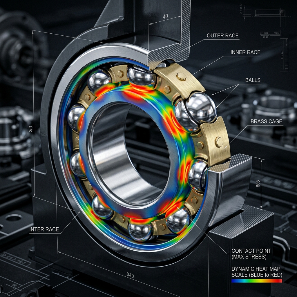
Fatigue Design and Contact Mechanics of Rolling Element Bearings under Variable Dynamic Loading

Section 1: Introduction and Classification of Rolling Element Bearings

The historical evolution of rotating machinery is intimately linked with the development of bearing technology. The fundamental requirement of a bearing is to permit relative rotation between two components while transmitting mechanical loads with minimal frictional losses. Historically, sliding contact bearings (journal or sleeve bearings) served as the primary mechanism for supporting rotating shafts. In sliding bearings, the relative motion is accommodated by a thin layer of lubricant (fluid film lubrication) or direct sliding contact in boundary lubrication regimes. The coefficient of friction in such systems ranges from $\mu \approx 0.05$ under optimal hydrodynamic lubrication to $\mu \approx 0.1 - 0.2$ during start-up, shut-down, or transient overload conditions. The transition to rolling element bearings (REBs) replaced sliding motion with rolling motion, exploiting the physical principle that rolling resistance is orders of magnitude lower than sliding resistance. This innovation reduced the coefficient of friction to values between $\mu \approx 0.001$ and $0.005$, earning REBs the designation of "anti-friction" bearings.

However, the replacement of conforming sliding surfaces with non-conforming rolling geometries introduces a critical tribological trade-off. While sliding bearings distribute loads over a large surface area (yielding low nominal pressures), rolling element bearings transmit loads through micro-scale contact zones. For instance, the contact between a spherical ball and a curved inner raceway occurs theoretically at a single mathematical point, which deforms elastically under load into a microscopic ellipse. Consequently, the local contact stresses within these zones are exceptionally high, routinely reaching values between $1.0\text{ GPa}$ and $3.5\text{ GPa}$. Under cyclic loading, these localized stress fields cause cumulative micro-structural damage to the bearing material, culminating in Rolling Contact Fatigue (RCF). RCF is characterized by subsurface crack initiation, propagation, and eventual material detachment (spalling or flaking), which serves as the primary limiting factor for the service life of a properly lubricated and sealed bearing.

To prevent premature wear and excessive friction, REBs rely on the mechanics of Elastohydrodynamic Lubrication (EHL). EHL represents a specialized lubrication regime where two physical phenomena occur simultaneously: first, the extreme pressures within the contact zone cause an exponential increase in the lubricant's viscosity (the piezo-viscous effect, typically modeled using Barus' relation $\eta = \eta_0 e^{\alpha p}$, where $\alpha$ is the pressure-viscosity coefficient); second, the contacting metal surfaces undergo significant elastic deformation. Under EHL, a thin, highly pressurized oil film (typically on the order of $0.1$ to $1.0\ \mu\text{m}$) is entrained into the contact zone, separating the surface asperities. The thickness of this film is mathematically described by minimum film thickness equations, such as the classical Dowson-Higginson formula for line contact:

where $U$ is the dimensionless speed parameter, $G$ is the dimensionless materials parameter, $W$ is the dimensionless load parameter, and $R'$ is the equivalent radius of curvature. A critical insight from EHL theory is that the film thickness is highly sensitive to rotational speed and oil viscosity, but almost independent of the applied load. The ratio of this film thickness to the composite surface roughness of the contacting bodies is defined as the film parameter:

where $\sigma_1$ and $\sigma_2$ are the root-mean-square (RMS) surface roughness values of the rolling element and the raceway, respectively. In engineering practice, maintaining $\Lambda > 3$ is required to ensure full-film lubrication, whereas operation at $\Lambda < 1$ leads to boundary lubrication, accelerating fatigue wear and micropitting.

1.1 Deep-Groove Ball Bearings (DGBBs)

Deep-groove ball bearings (DGBBs) are the most common type of rolling element bearing. They consist of an inner ring, an outer ring, a set of spherical balls, and a cage. The cage physically separates the balls to prevent contact-induced friction and wear, and to guide them through the loaded and unloaded zones. The defining geometric parameter of a DGBB is the groove geometry of the raceways, which is characterized by the osculation ratio $f$. Osculation is the ratio of the transverse groove radius of curvature $r_g$ to the ball diameter $D_w$:

where $r_i$ and $r_o$ represent the groove radii of the inner and outer raceways, respectively. For standard commercial bearings, the osculation ratio is typically designed between $0.515$ and $0.530$. If the osculation is too close to $0.50$ (highly conforming contact), the contact area becomes large, increasing the frictional torque and heat generation due to differential sliding (Heathcote slip). If $f$ is too large (e.g., $> 0.54$, indicating poor conformance), the contact area decreases, elevating the local Hertzian contact stress and reducing the fatigue life.

Under purely radial loads, the nominal contact angle $\alpha_0$ of a DGBB is zero. In this state, the contact forces are perpendicular to the shaft axis. However, because the groove depth is significant, the balls are laterally guided. When subjected to an axial (thrust) load $F_a$, the inner and outer rings shift axially relative to each other, causing the balls to climb the groove sides. This displacement changes the contact angle from its nominal value of $0^\circ$ to an operational contact angle $\alpha > 0^\circ$. Consequently, DGBBs possess a bidirectional axial load-carrying capacity in addition to their radial capacity. The magnitude of this axial capacity is limited by the radial clearance and the shoulder height of the grooves, which must be high enough to prevent the contact ellipse from overriding the edge of the raceway.

1.2 Cylindrical Roller Bearings (CRBs)

Cylindrical roller bearings (CRBs) utilize cylinders as rolling elements instead of spheres. This structural difference alters the fundamental nature of the contact mechanics: whereas ball bearings exhibit point contact (which deforms into an elliptical patch under load), cylindrical roller bearings exhibit line contact (which deforms into a rectangular patch). The primary consequence of line contact is a significantly larger load transmission area, which dramatically increases the radial load capacity of CRBs compared to DGBBs of equivalent dimensions.

However, the kinematics of cylindrical rollers impose constraints on axial load transmission. Because the contact angle is strictly $\alpha = 0^\circ$ and cannot shift under load, a standard CRB (e.g., NU or N type) cannot transmit axial loads. Any axial force would cause the rollers to slide along the cylindrical raceways. To accommodate axial forces, CRBs are configured with integral ribs (flanges) on the inner and outer rings (e.g., NJ, NUP, or NH types). Under axial load, the axial force is transmitted via sliding contact between the end faces of the rollers and the radial guide surfaces of the ribs. Since this contact is sliding rather than rolling, it is highly susceptible to adhesive wear (scuffing) and thermal distress, requiring careful attention to lubricant viscosity and supply.

A major vulnerability of line contact is its sensitivity to angular misalignment. If the shaft deflects or is misaligned relative to the housing, the load is no longer distributed uniformly along the length of the roller. Instead, the load concentrates at the roller ends, a phenomenon known as edge loading. Theoretically, the sharp boundary at the ends of an ideal cylinder contacting a flat surface yields a stress singularity. To eliminate these destructive edge stresses, modern roller bearings employ crowned rollers. The profile of the roller is slightly curved along its longitudinal axis, deviating from a perfect cylinder. While circular crowning (a simple large radius) is common, advanced high-capacity bearings utilize a logarithmic profile, which is mathematically optimized to yield a uniform stress distribution along the contact length under the design load.

1.3 Spherical Roller Bearings (SRBs)

Spherical roller bearings (SRBs) are specifically engineered to operate under conditions of extreme radial loads, substantial axial loads, and severe shaft misalignment or deflection. The classic design of an SRB consists of two rows of barrel-shaped rollers (symmetrical or asymmetrical), an inner ring with two inclined raceways, and an outer ring with a single, continuous spherical raceway. The center of curvature of the outer ring’s spherical surface lies on the rotation axis of the bearing.

This unique spherical geometry provides the bearing with its self-aligning capability. If the shaft bends under load or experiences angular misalignment during installation (up to $1.5^\circ$ to $2.5^\circ$), the inner ring, cage, and rollers can tilt as a unit within the outer ring without generating edge stresses. The rollers maintain conforming contact with the spherical outer raceway and the inclined inner raceways.

The load transmission path in an SRB is inclined at an angle to the radial plane, which means each row of rollers has a distinct contact angle $\alpha$. Because of this inclination, SRBs can support very large radial forces combined with significant bidirectional thrust loads. The barrel shape of the rollers results in point contact at zero load, which rapidly transitions to elliptical contact under operational loads. The design of the cage and the presence of a floating guide ring between the two roller rows are critical in ensuring that the rollers do not skew (rotate about their radial axis) as they enter and exit the loaded zone.

1.4 Tapered Roller Bearings (TRBs)

Tapered roller bearings (TRBs) are designed to handle heavy combined radial and thrust loads. The structural components of a TRB include an inner ring (cone), an outer ring (cup), tapered rollers, and a cage. The defining geometric principle of a TRB is that the conical surfaces of the raceways and the rollers are designed with a common apex.

Mathematically, the projection of the conical surfaces of the cup, cone, and the tapered rollers must intersect at a single point on the rotational axis of the bearing, known as the apex point. This geometric condition ensures that true rolling contact occurs at every point along the length of the roller. Because the linear speed of a point on the cone surface increases with its radius, the roller diameter must increase proportionally along its length. By aligning the cones to a single apex, the relative sliding velocity between the roller surface and the raceways is theoretically zero, preventing frictional losses and wear along the contact line.

Under radial or axial load, the tapered geometry generates a seating force that pushes the rollers against the large rib on the inner ring (cone). The contact between the large end face of the roller and this rib is a sliding contact, which must be lubricated to prevent scuffing. Due to the contact angle $\alpha$, a purely radial load $F_r$ will generate an induced axial force:

where $Y$ is the axial load factor of the bearing. To balance this induced thrust force, TRBs are almost always mounted in pairs (either back-to-back, DB, or face-to-face, DF) or as double-row units. Adjusting the axial clearance during mounting (preloading) is essential to establish the correct contact stress distribution and optimize system stiffness.

1.5 Needle Roller Bearings (NRBs)

Needle roller bearings (NRBs) are a specialized sub-category of cylindrical roller bearings characterized by rolling elements with a high aspect ratio. Specifically, needle rollers are thin cylinders where the ratio of the length $L_w$ to the diameter $D_w$ is equal to or greater than 3, and typically ranges up to 10:

The primary engineering advantage of NRBs is their exceptionally compact radial cross-section. For applications where radial space is severely restricted (such as transmission gearboxes, universal joints, and small engine connecting rods), NRBs provide a radial height that is comparable to a simple sliding bushing, while maintaining the low friction and high starting torque characteristics of rolling contact.

Despite their high radial load capacity, NRBs possess unique kinematic vulnerabilities. Because the rollers are long and thin, they are highly flexible and susceptible to bending under non-uniform loads. Furthermore, any small alignment error or manufacturing tolerance deviation can cause roller skewing, where the roller axis rotates out of alignment with the bearing axis. Skidding and skewing generate high sliding friction against the cage or adjacent rollers, leading to rapid heat generation and cage failure. Consequently, precise roller guidance via a rigid cage or accurately ground shaft and housing surfaces (when operating without separate inner or outer rings) is critical.

1.6 High-Performance Applications

1.6.1 Space Applications: Cryogenic Turbopumps

In space propulsion systems, such as the liquid hydrogen ($\text{LH}_2$) and liquid oxygen ($\text{LOX}$) turbopumps of rocket engines (e.g., the Space Shuttle Main Engine or Merlin engines), bearings must operate under extreme environmental conditions. These turbopumps rotate at speeds exceeding $20,000$ to $100,000\text{ rpm}$ while submerged in cryogenic fluids ($\text{LH}_2$ at $20\text{ K}$ or $\text{LOX}$ at $90\text{ K}$).

Cryogenic liquids have extremely low viscosity (liquid hydrogen has a viscosity lower than water), which prevents the formation of a conventional elastohydrodynamic lubricant film. To survive under these conditions, hybrid ceramic bearings are utilized. These bearings feature rings made from advanced corrosion-resistant, high-nitrogen stainless steel (such as Cronidur 30) paired with rolling elements made of Silicon Nitride ($\text{Si}_3\text{N}_4$) ceramic. The ceramic balls offer several advantages: they are $40\%$ less dense than steel (reducing centrifugal forces at high speeds), have a higher elastic modulus (increasing stiffness), and exhibit a very low coefficient of thermal expansion, preventing thermal seizure. Because liquid oxygen is highly reactive, standard hydrocarbon lubricants cannot be used. Instead, solid lubrication is employed. The cages are fabricated from self-lubricating polymer composites containing polytetrafluoroethylene (PTFE) or molybdenum disulfide ($\text{MoS}_2$), which transfer a microscopic solid film to the balls and raceways during operation. Vacuum operations also dictate strict outgassing controls, as volatile components of standard grease would vaporize and contaminate sensitive optical and electronic sensors.

1.6.2 Aerospace Applications: Aircraft Gas Turbines

The mainshaft bearings of aircraft jet engines support the high-pressure and low-pressure compressor and turbine shafts. These bearings operate at high speeds, typically characterized by a speed index ($DN$ value) of:

where $d$ is the bore diameter in millimeters and $n$ is the rotational speed in rpm. At these velocities, centrifugal forces and gyroscopic moments acting on the rolling elements dominate the stress state, altering the contact angles at the inner and outer races.

To withstand the high temperatures (up to $250^\circ\text{C}$) and cyclic stresses, these bearings are manufactured from premium tool steels such as M50 or case-hardened M50-NiL. The lubrication system must actively cool the bearing. Rather than simple splash lubrication, oil-jet or under-race lubrication is employed. In under-race lubrication, centrifugal force pumps synthetic oil through radial holes in the inner ring directly into the contact zone. Furthermore, to mitigate the vibrations caused by rotor imbalance and high-speed dynamics, the outer rings of the bearings are often mounted inside a squeeze film damper (SFD)—a thin annular oil cavity that provides hydrodynamic damping to the rotor-bearing assembly.

1.6.3 Heavy Industrial Applications: Wind Turbine Main Shafts

In contrast to high-speed aerospace applications, wind turbine main shaft bearings operate at very low speeds ($8$ to $20\text{ rpm}$) but are subjected to massive, highly variable, and unpredictable aerodynamic loads. Modern multi-megawatt wind turbines ($5$ to $15\text{ MW}$) utilize large-diameter spherical or tapered roller bearings (often exceeding $2\text{ meters}$ in diameter) to support the rotor.

Because of the low rotational speeds, the entrainment velocity of the lubricant is insufficient to generate a thick EHL film, causing the bearing to operate continuously in the boundary or mixed lubrication regime ($\Lambda < 1$). Under these conditions, the surface asperities contact each other, leading to adhesive wear and micropitting. Moreover, wind turbine bearings are susceptible to a structural failure mode known as White Etching Cracks (WECs). WECs are networks of subsurface microcracks surrounded by a microstructural alteration (ferrite recrystallization) that appears white under acid etching. These cracks propagate under the influence of cyclic contact stresses, electrical currents (from generator discharge), and hydrogen embrittlement (from lubricant decomposition), leading to premature and catastrophic bearing failure. To prevent this, heavy industrial bearings are coated with black oxide or specialized tungsten carbide carbon (WCC) coatings, and are lubricated with high-viscosity greases formulated with specialized extreme pressure (EP) and anti-wear (AW) additives.

Section 2: Contact Mechanics and Hertzian Stress Derivations

2.1 Fundamentals of Elastic Contact Theory

The mathematical analysis of contact stresses between non-conforming elastic bodies originates from the pioneering work of Heinrich Hertz in 1881. The classical Hertzian contact theory relies on several simplifying assumptions, which must hold to ensure the validity of the stress derivations:

1. The contacting materials are homogeneous, isotropic, and exhibit linear elastic behavior conforming to Hooke's Law.
2. The contact surfaces are frictionless, meaning only normal forces are transmitted across the interface, and shear stresses ($\tau_{xz}, \tau_{yz}$) on the surface are zero.
3. The dimensions of the contact area (e.g., semi-axes $a$ and $b$) are very small compared to the characteristic radii of curvature of the contacting bodies. This allows the contacting bodies to be modeled as infinite elastic half-spaces.
4. The contact is non-conforming, meaning the initial contact under zero load is either a point or a line.

2.2 Geometry of Contacting Bodies in Three Dimensions

Consider two elastic bodies, designated as Body 1 and Body 2, which are brought into contact at a point. Let us establish a global Cartesian coordinate system where the origin $O$ coincides with the initial point of contact. The $z$-axis is oriented normal to the tangent plane of the contacting surfaces, pointing into Body 1, while the $x$ and $y$ axes lie within the tangent plane.

The profile of each surface $i$ ($i=1, 2$) in the immediate vicinity of the origin can be mathematically represented using a Taylor series expansion, truncated to the second order:

By rotating the coordinate system about the $z$-axis through an angle $\phi$, we can eliminate the cross-product terms ($xy$). In this principal coordinate frame, the distance $z$ separating the two surfaces before deformation is given by:

where the constants $A$ and $B$ are geometric parameters defined by the principal curvatures of the two bodies. Let the principal curvatures (inverse of the radii of curvature) of Body 1 be $k_{11} = 1/r_{11}$ and $k_{12} = 1/r_{12}$, and those of Body 2 be $k_{21} = 1/r_{21}$ and $k_{22} = 1/r_{22}$. The coefficients $A$ and $B$ are related to these curvatures by:

Here, $\phi$ is the angle between the plane containing the principal curvature $k_{11}$ of Body 1 and the plane containing the principal curvature $k_{21}$ of Body 2. For rolling element bearings, the principal planes of curvature of the rolling elements and raceways are aligned, meaning $\phi = 0$. Under this alignment, the curvature difference simplifies to:

The sum of the curvatures $\sum \rho$ is a critical parameter:

To characterize the eccentricity of the contact area, we define the curvature difference parameter $F(\rho)$ as:

The mechanical compliance of the contact is governed by the equivalent elastic modulus $E^*$ (reduced modulus), which accounts for the elastic properties (Young's modulus $E$ and Poisson's ratio $\nu$) of both contacting bodies:

2.3 Mathematical Derivation for Point Contact (Elliptical Contact)

When two bodies with double curvature are pressed together with a normal force $F$, the contact area is an ellipse with semi-major axis $a$ and semi-minor axis $b$ ($a \ge b$). According to potential theory, the elastic displacement $w_1(x, y)$ and $w_2(x, y)$ of the two bodies within the contact zone must satisfy the kinematic condition of contact:

where $\delta$ is the mutual approach (deflection) of distant points in the two bodies. The displacement of a point on the surface of an elastic half-space subjected to a normal pressure distribution $p(x', y')$ is given by the Boussinesq integral:

Substituting this into the kinematic condition yields the fundamental integral equation of contact mechanics:

Hertz postulated that the pressure distribution that satisfies this integral equation is semi-ellipsoidal:

where $p_0$ is the maximum contact pressure at the center of the contact. To relate the total force $F$ to the maximum pressure, we integrate the pressure distribution over the elliptical domain $\Omega$:

Using the coordinate transformation $x = a r \cos\theta$ and $y = b r \sin\theta$, the Jacobian of the transformation is $J = a b r$. The integral becomes:

This yields the relation for the maximum contact pressure:

By evaluating the potential of the ellipsoid, the semi-axes $a$ and $b$ are expressed in terms of the complete elliptic integrals of the first kind $K(e)$ and second kind $E(e)$:

where the eccentricity of the contact ellipse is $e = \sqrt{1 - (b/a)^2}$. The equations linking the geometry to the elliptic integrals are:

The dimensions $a$ and $b$, and the deformation $\delta$ are determined using transcendental coefficients $a^*$, $b^*$, and $\delta^*$:

where the dimensionless coefficients are defined as:

Because solving these transcendental equations analytically is difficult, engineers utilize the accurate approximations developed by Hamrock and Dowson. Let the ratio of the principal curvatures be defined as $\kappa = B/A$. The elliptical eccentricity parameter $k_e = a/b$ can be approximated by:

The elliptic integrals can be approximated as functions of $k_e$:

2.3.1 Subsurface Stress Field Derivation

Rolling contact fatigue is driven by the subsurface stress field beneath the contact patch. Along the normal axis of symmetry ($z$-axis), the principal stresses $\sigma_x$, $\sigma_y$, and $\sigma_z$ are compressive. For a circular contact area ($a = b = r$), the analytical stress equations along the $z$-axis are:

The maximum shear stress $\tau_{\text{max}}$ is defined as:

Evaluating this for steel ($\nu = 0.3$) shows that $\tau_{\text{max}}$ reaches a peak value of:

However, in rolling contacts, the material is subjected to a moving stress field. The orthogonal shear stress $\tau_{yz}$ (or $\tau_{xz}$ in the direction of rolling) acts in planes parallel and perpendicular to the contact surface. As a rolling element passes over a point on the raceway, the orthogonal shear stress undergoes a complete reversal:

The maximum value of this reversing orthogonal shear stress is $\tau_{0} \approx 0.25 p_0$ to $0.28 p_0$, occurring at a shallower depth of $z \approx 0.35 b$ and laterally shifted by $y \approx 0.35 b$. Because of this alternating, fully reversed loading, the orthogonal shear stress is critical in the Lundberg-Palmgren fatigue model for predicting crack initiation.

2.4 Mathematical Derivation for Line Contact (Rectangular Contact)

For cylindrical rollers contacting a cylindrical raceway, the contact zone is represented by a rectangle of width $2b$ and length $L$ ($L \gg b$). The pressure distribution is semi-cylindrical across the width:

Integrating the pressure across the contact width to balance the total normal force $F$:

This gives the relation for the maximum line contact pressure:

The contact half-width $b$ is derived by matching the deformation to the profile of the cylinder. Using the plane strain approximation for an infinite cylinder:

where $R'$ is the equivalent radius of curvature of the roller-raceway pair:

Substituting the expression for $b$ back into the formula for $p_0$ yields the maximum contact stress as a function of load:

Calculating the elastic deflection $\delta$ under line contact is more complex than in point contact. Because the displacement field under a line load does not decay to zero at infinity, a reference boundary condition is required. A widely accepted empirical equation for the deflection of steel cylinders in contact is Palmgren's formula:

Alternatively, Houpert's analytical formulation defines the deflection as:

2.4.1 Subsurface Stress Field in Line Contact

The subsurface stress field along the normal $z$-axis beneath a line contact is given by:

The maximum shear stress $\tau_{\text{max}} = \frac{1}{2}|\sigma_z - \sigma_y|$ for steel ($\nu = 0.3$) reaches its peak value of:

This deeper location of the maximum shear stress compared to point contact ($z \approx 0.47 a$) is an important consideration in material selection and heat treatment, requiring a deeper case-hardening depth for roller bearings.

2.5 Corrections for Real Roller Geometry (Crowning)

The ideal line contact equations assume that the cylinder is infinitely long or that the contact stress drops to zero at the boundary. In real, finite-length cylindrical rollers, the discontinuity at the roller ends causes local stress concentrations. In a roller with a straight profile, this edge-loading effect creates a theoretical stress singularity at the corners, which accelerates fatigue and leads to end-peeling.

To prevent this, modern rollers are crowned. Circular crowning introduces a large, continuous radius $R_c$ (typically $R_c \approx 100 \times$ to $1000 \times$ the roller radius) along the longitudinal profile. While circular crowning reduces edge stresses, it can lead to high center stresses under heavy loads.

The optimal profile is the logarithmic profile, derived by Johns and Gohar. The profile drop $z(x)$ as a function of the axial coordinate $x$ (measured from the roller center) is defined as:

where $l$ is the half-length of the contact, $p_0$ is the design contact pressure, and $R'$ is the equivalent radius of curvature. Because this profile drop approaches infinity as $x \to l$, practical manufacturing designs utilize a modified logarithmic profile. These profiles are manufactured using precision grinding to achieve a uniform stress distribution across the entire roller length under the design load.

Section 3: Dynamic Equivalent Load & Kinematics

3.1 Dynamic Load Ratings (Lundberg-Palmgren Theory)

The dynamic load rating of a rolling element bearing is based on the statistical model of rolling contact fatigue developed by Lundberg and Palmgren. This model links the probability of survival $S$ of a volume of material to the critical subsurface shear stress $\tau_0$, the depth $z_0$ at which this stress occurs, the number of stress cycles $N$ (in millions of revolutions), and the volume $V$ subjected to high stress. This relationship is expressed using a Weibull distribution:

where $e$ is the Weibull slope (slope of the dispersion of life values), and $c$ and $h$ are material exponents determined experimentally. For bearing steel, the exponents are typically $e = 10/9$ for ball bearings and $e = 9/8$ for roller bearings.

The Basic Dynamic Load Rating $C$ is defined as the constant load that a bearing can support for a nominal rating life of one million revolutions ($N=1$) with a $90\%$ probability of survival ($S=0.9$). Based on this definition, the rating life $L_{10}$ in millions of revolutions is given by:

where $P$ is the dynamic equivalent load, and the life exponent $p$ depends on the contact geometry:

• For ball bearings (point contact), $p = 3$. This exponent reflects the cubic relationship between stress and load, where the contact area increases as $F^{2/3}$ and the maximum pressure $p_0$ increases as $F^{1/3}$.
• For roller bearings (line contact), $p = 10/3 \approx 3.333$. This higher exponent reflects the line contact geometry, where the contact width increases as $F^{1/2}$ and the maximum pressure $p_0$ increases as $F^{1/2}$.

3.2 Dynamic Equivalent Load Derivation

Bearings in service are often subjected to combined radial ($F_r$) and axial ($F_a$) loads. To evaluate the fatigue life of the bearing, these combined forces must be converted into a single virtual load that would produce the same fatigue life as the actual combined load. This virtual load is the Dynamic Equivalent Load $P$, expressed as:

where $X$ is the radial load factor and $Y$ is the axial load factor. The values of $X$ and $Y$ depend on the contact angle $\alpha$ and the ratio of axial to radial force.

This relationship is derived from the load distribution within the bearing. Let $\psi$ represent the angular position of a rolling element, with $\psi = 0$ corresponding to the most heavily loaded element at the center of the loaded zone. The load $q(\psi)$ on any rolling element at position $\psi$ can be described using Sjövall's distribution:

where $\epsilon$ is the load distribution parameter, $q_{\text{max}}$ is the maximum rolling element load, and the exponent $n$ is $1.5$ for ball bearings and $1.0$ for roller bearings. The parameter $\epsilon$ determines the extent of the loaded zone: $\epsilon = 0.5$ indicates a loaded zone of exactly $180^\circ$, while $\epsilon > 0.5$ indicates a larger loaded zone, and $\epsilon < 0.5$ represents a narrower loaded zone.

The total radial force $F_r$ and axial force $F_a$ are obtained by integrating the individual rolling element forces over the loaded zone:

where $Z$ is the number of rolling elements, and $J_r(\epsilon)$ and $J_a(\epsilon)$ are the Sjövall integrals:

Here, $\pm\psi_l$ represents the angular limits of the loaded zone. The ratio of the forces is:

When the axial force is small relative to the radial force ($F_a / F_r \le e$, where $e$ is a threshold parameter proportional to $\tan\alpha$), the loaded zone is primarily radial. Under these conditions, the axial load does not significantly alter the stress distribution, and the equivalent load is determined solely by the radial load ($X=1, Y=0$, so $P = F_r$).

When $F_a / F_r > e$, the axial load shifts the contact zone and increases the maximum contact stresses. Under these conditions, the axial component must be accounted for using the factors $X < 1$ and $Y > 1$ (e.g., $P = 0.56 F_r + Y F_a$ for DGBBs, where $Y$ varies with the contact angle and axial force).

3.2.1 Variable Dynamic Loading and Damage Accumulation

In many industrial applications, bearings operate under loads that vary over time. To analyze fatigue life under variable loading, the linear damage accumulation theory (Palmgren-Miner Rule) is applied. This rule states that the total fatigue damage $D$ is the sum of the cycle ratios:

where $n_i$ is the number of revolutions accumulated under load $P_i$, and $L_i$ is the rating life corresponding to that load. Fatigue failure is predicted to occur when the damage sum reaches unity ($D = 1$).

For a bearing subjected to a series of discrete load steps $P_i$, each acting for $n_i$ revolutions, the equivalent dynamic load $P_{\text{eq}}$ over the total number of revolutions $N = \sum n_i$ is:

For a continuously varying load history $P(t)$ over an operating period $T$, this relationship is expressed in integral form:

where $p=3$ for ball bearings and $p=10/3$ for roller bearings.

3.3 Kinematics of Rolling Element Bearings

The kinematics of rolling element bearings govern the velocities of the internal components under the assumption of pure rolling contact (no slip). Let us define the following geometric parameters:

• $d_m$: Pitch diameter of the rolling element set, measured from the centers of the elements.
• $D_w$: Diameter of the rolling elements.
• $\alpha$: Operating contact angle.
• $n_i$ and $n_o$: Rotational speeds (in rpm) of the inner and outer rings, respectively.

3.3.1 Derivation of Cage Speed

Under the assumption of pure rolling, the linear velocity of the contact point on the inner ring is:

Similarly, the linear velocity of the contact point on the outer ring is:

Since the cage supports the centers of the rolling elements, the linear velocity $v_c$ of the cage at the pitch diameter is the average of the velocities of the inner and outer contact points:

The rotational speed of the cage $n_c$ (in rpm) is related to its linear velocity by $v_c = \pi n_c d_m$. Substituting this relationship yields the general equation for cage speed:

For the common case where the outer ring is stationary ($n_o = 0$), this simplifies to:

3.3.2 Derivation of Rolling Element Rotational Speed

The rotational speed $n_w$ of a rolling element about its own axis is determined by the relative velocity between the cage and the races. The relative linear velocity at the inner race contact point is:

Under pure rolling, this relative velocity equals the peripheral speed of the rolling element:

Equating these two expressions and solving for $n_w$ yields:

Taking the magnitude of this speed for a stationary outer ring ($n_o = 0$):

3.3.3 Derivation of Kinematic Defect Frequencies

In vibration-based condition monitoring, localized defects on the bearing components (inner race, outer race, rolling elements, or cage) generate periodic vibration impulses. The frequencies of these impulses are determined by the bearing kinematics. Let $f_i$ and $f_o$ represent the rotational frequencies (in Hz) of the inner and outer rings ($f = n/60$). The defect frequencies are defined as follows:

• Ball Pass Frequency Outer (BPFO): The frequency at which rolling elements pass over a single point on the outer raceway.
  $$ f_{\text{BPFO}} = \frac{Z}{2} |f_i - f_o| \left( 1 - \frac{D_w}{d_m}\cos\alpha \right) $$
• Ball Pass Frequency Inner (BPFI): The frequency at which rolling elements pass over a single point on the inner raceway.
  $$ f_{\text{BPFI}} = \frac{Z}{2} |f_i - f_o| \left( 1 + \frac{D_w}{d_m}\cos\alpha \right) $$
• Fundamental Train Frequency (FTF): The rotational frequency of the cage assembly.
  $$ f_{\text{FTF}} = \frac{1}{2} \left[ f_i \left( 1 - \frac{D_w}{d_m}\cos\alpha \right) + f_o \left( 1 + \frac{D_w}{d_m}\cos\alpha \right) \right] $$
• Ball Spin Frequency (BSF): The rotational frequency of a rolling element about its own axis, determining the rate at which a defect on the element contacts either the inner or outer raceway.
  $$ f_{\text{BSF}} = \frac{d_m}{2 D_w} |f_i - f_o| \left[ 1 - \left( \frac{D_w}{d_m}\cos\alpha \right)^2 \right] $$

3.4 Slip and Skidding Phenomena

The assumption of pure rolling contact is a simplification. In real applications, rolling elements experience localized sliding, which can be categorized into micro-slip and macro-slip.

Heathcote Slip is a form of micro-slip that occurs because the contact area between a ball and a curved groove is curved rather than flat. The distance from the ball's axis of rotation to the contact surface varies across the contact ellipse, meaning the local rolling radius varies. Consequently, pure rolling can only occur at two symmetric bands within the contact ellipse. In the regions between and outside these bands, the surfaces must slide relative to each other, generating friction, heat, and sliding wear.

Skidding is a form of macro-slip that occurs in high-speed, lightly loaded bearings (such as jet engine mainshaft bearings). Under these conditions, the centrifugal force on the rolling elements increases, but the radial force is insufficient to maintain the tractive force required to drive the cage and rollers at their theoretical kinematic speeds. As a result, the rolling elements slide or skid against the inner raceway. Skidding breaks down the EHL film, leading to metal-to-metal contact, adhesive wear (scuffing), and thermal damage that can cause rapid bearing failure.

Section 4: Numerical Worked Example

To bridge the gap between abstract mathematical models and practical mechanical engineering, this section presents a comprehensive, step-by-step fatigue design calculation for a tapered roller bearing (TRB) operating in the main generator shaft of a 3.0 MW wind turbine. Tapered roller bearings are highly preferred in wind turbine generator shafts due to their unique capability to support large simultaneous radial and axial loads. They also provide high system rigidity, and their preload can be adjusted during assembly to minimize shaft deflection under dynamic loading. However, wind turbine drivetrains are subjected to highly variable wind speeds, wind shears, and aerodynamic transients (such as gusts and emergency shutdowns), which impose complex, non-stationary load-speed profiles on the bearing. To prevent premature failure, a design engineer must evaluate the cumulative fatigue damage under a variable duty cycle. In this worked example, we will calculate the nominal rating life ($L_{10h}$) under a multi-bin duty cycle, apply Palmgren-Miner's rule for cumulative damage, synthesize the results using equivalent load and speed methods, and finally evaluate the modified reference life ($L_{10mh}$) according to the ISO 281 standard.

4.1 Bearing Geometry and Technical Specifications

The bearing selected for this generator shaft application is a double-row tapered roller bearing. Its primary design parameters, dynamic load ratings, and geometric characteristics are summarized in the table below. Tapered roller bearings feature conical rollers and raceways, meaning the contact lines of the rollers and raceways intersect at a common point on the bearing axis (the apex). This geometry ensures true rolling motion of the rollers at all points along the contact line, eliminating sliding friction and reducing heat generation. The contact angle $\alpha$ determines the ratio of radial to axial load-carrying capacity; a larger contact angle increases the thrust capacity but reduces the radial capacity.

Table 4.1: Double-Row Tapered Roller Bearing Parameters

4.2 Wind Turbine Duty Cycle and Load Spectrum

A representative generator-shaft duty cycle, divided into four discrete operational bins, has been compiled from supervisory control and data acquisition (SCADA) systems and aeroelastic simulation models (e.g., NREL FAST). Each bin represents a specific environmental/wind state, with corresponding shaft rotational speeds ($n_i$), radial shaft loads ($F_{r,i}$), axial generator-thrust loads ($F_{a,i}$), and the relative time fraction ($q_i$) that the turbine spends in that state over its lifetime.

Table 4.2: Generator Shaft Bearing Load-Speed Spectrum

4.3 Bin-by-Bin Equivalent Dynamic Load and Nominal Life Calculations

To evaluate the fatigue life of the bearing under variable load combinations, we must first calculate the equivalent dynamic load ($P_i$) for each operating bin. For tapered roller bearings, the equivalent load is calculated by comparing the ratio of the axial load to the radial load ($F_a / F_r$) with the threshold factor $e$. This step-by-step load combination accounts for the contact angle mechanics, in which the radial load induces an axial force that must be balanced by the axial load.

The mathematical formulas for equivalent dynamic load are defined as follows:

Once $P_i$ is determined, the nominal dynamic rating life in millions of revolutions ($L_{10,i}$) and in hours ($L_{10h,i}$) for each bin is calculated using the following relations:

We now proceed with the step-by-step arithmetic calculations for each of the four bins:

Bin 1: Low Wind / Cut-in
1. Calculate the load ratio:

Bin 2: Below-Rated Operation
1. Calculate the load ratio:

Bin 3: Rated Wind Operation
1. Calculate the load ratio:

Bin 4: High Wind Aerodynamic Gust / Transient
1. Calculate the load ratio:

4.4 Damage Accumulation via Palmgren-Miner's Rule

Under variable loading conditions, fatigue damage accumulates in the material of the rollers and raceways. According to the Palmgren-Miner linear damage hypothesis, the cumulative fatigue damage ($D_{tot}$) accumulated per hour is the sum of the cycle ratios (fraction of time spent in a bin divided by the bearing life in hours for that bin). The physical assumption is that each revolution consumed at a given load takes a linear fraction of the total life available at that load, independent of the loading history sequence.

The total damage per hour is expressed as:

Substituting the calculated lives and time fractions from our load spectrum, we obtain the total damage per hour:

Evaluating each term:
- Low Wind Damage: $D_1 = 1.2083 \times 10^{-5}\text{ hours}^{-1}$ (or $0.41\%$ of total damage)
- Below-Rated Damage: $D_2 = 2.5146 \times 10^{-4}\text{ hours}^{-1}$ (or $8.49\%$ of total damage)
- Rated Wind Damage: $D_3 = 6.1363 \times 10^{-4}\text{ hours}^{-1}$ (or $20.72\%$ of total damage)
- Transient Damage: $D_4 = 2.0845 \times 10^{-3}\text{ hours}^{-1}$ (or $70.38\%$ of total damage)

Summing these damage components yields:

The total nominal system fatigue life ($L_{10h,\text{sys}}$) is the reciprocal of the total hourly damage rate:

The calculation highlights a crucial dynamic in wind turbine reliability: even though the turbine spends only $10\%$ of its operational life in the gust/transient condition (Bin 4), this state accounts for over $70\%$ of the total dynamic fatigue damage. This is a direct consequence of the cubic-like exponent ($p = 10/3$) of roller bearings, where any increase in dynamic loading is amplified exponentially.

4.5 Synthesis via Equivalent Operating Conditions

An alternative method commonly employed by bearing manufacturers is to replace the variable duty cycle with a single equivalent rotational speed ($n_{eq}$) and a single equivalent dynamic load ($P_{eq}$) that result in the exact same cumulative fatigue life.

The equivalent speed is the linear time-weighted average of the speeds:

The equivalent dynamic load is a weighted average of the loads, where the weighting factor is the product of speed and time fraction, raised to the exponent $1/p$:

We calculate $n_{eq}$ and $P_{eq}$ as follows:
1. Calculate equivalent speed:

4.6 Design Optimization for 20-Year Operational Lifetime

The calculated nominal fatigue life of $337.65$ hours is extremely short for a wind turbine generator shaft. In industrial wind energy applications, drivetrains are designed for a 20-year or 30-year operational lifetime. A typical target fatigue life for a bearing of this class is $L_{10h,req} = 175,000$ hours (approximately 20 years of continuous operation, allowing for maintenance downtimes).

To achieve this target life, the dynamic load rating $C$ must be increased. We can calculate the required dynamic load rating ($C_{req}$) using the equivalent speed ($n_{eq}$) and equivalent load ($P_{eq}$):

Substituting our values:

This calculation reveals that a dynamic load rating of approximately $12,109\text{ kN}$ is required. In engineering practice, this is achieved by using a much larger bearing, using multiple rows of rollers (e.g., four-row tapered roller bearings), increasing the roller length and diameter, or implementing an active load-sharing lubrication system that reduces the peak loads. However, increasing the bearing size increases the rotating mass, cost, and frictional torque. Frictional torque in bearings is a significant source of power loss in wind turbines, which must be balanced against fatigue life.

4.7 ISO 281 Life Modification Factors ($L_{10m}$)

The nominal $L_{10}$ calculation assumes standard clean operating conditions and full elastohydrodynamic film separation. In reality, bearing life is heavily modified by lubrication quality and oil cleanliness. The ISO 281 standard introduces the modified reference rating life $L_{nm}$, which incorporates reliability ($a_1$) and a life modification factor ($a_{ISO}$):

For our analysis, we assume a standard $90\%$ reliability ($a_1 = 1.0$). The life modification factor $a_{ISO}$ is a function of the contamination factor ($e_c$), the viscosity ratio ($\kappa = \nu / \nu_1$), and the fatigue load limit ratio ($P_u / P$). The viscosity ratio $\kappa$ represents the quality of the lubricating film: a high value indicates a thick film that separates the metal surfaces, whereas a low value indicates asperity contact.

For this worked example, we assume:
- Viscosity ratio: $\kappa = 2.5$ (indicating high-viscosity oil that provides good film separation).
- Contamination factor: $e_c = 0.6$ (representing a high-quality filter system with typical ISO 4406 cleanliness class 18/15/12, where particles are mostly filtered out).

Using the standard ISO 281 curves/equations for roller bearings, we calculate the parameter $\frac{e_c P_u}{P_i}$ for each bin and retrieve the corresponding $a_{ISO, i}$ factors:

Table 4.3: ISO 281 Life Modification Factors

Using Miner's Rule on these modified lives, the cumulative modified life $L_{10mh,\text{sys}}$ is calculated:

Evaluating each term:
- Low Wind Damage: $D_{1,m} = 2.685 \times 10^{-6}\text{ hours}^{-1}$
- Below-Rated Damage: $D_{2,m} = 1.676 \times 10^{-4}\text{ hours}^{-1}$
- Rated Wind Damage: $D_{3,m} = 7.671 \times 10^{-4}\text{ hours}^{-1}$
- Transient Damage: $D_{4,m} = 5.211 \times 10^{-3}\text{ hours}^{-1}$

Summing the modified damage rates:

The total modified reference rating life is:

This result demonstrates a critical physical mechanism in bearing mechanics: under heavy loads (such as Bins 3 and 4), the contact pressures are extremely high, causing the lubricant film to thin out and asperity contacts to increase. The modification factor $a_{ISO}$ drops below $1.0$ (to $0.80$ and $0.40$, respectively), which penalizes the lifetime. Conversely, under light loads (such as Bin 1), the film is thick enough to separate the surfaces, resulting in a large $a_{ISO}$ of $4.50$. However, because the heavy-load bins dominate the damage accumulation, the overall modified system life ($162.65\text{ hours}$) is actually shorter than the nominal system life ($337.65\text{ hours}$). This showcases why design engineers must evaluate the modification factor bin-by-bin rather than applying a single average $a_{ISO}$ factor.

Section 6: Lubrication Regime & Tribology

The fundamental objective of rolling element bearing lubrication is to minimize friction, wear, and heat generation by establishing a thin fluid film between the rolling elements and the raceways. Rolling element bearings operate under extremely high localized contact pressures, typically in the range of $1\text{ to }3\text{ GPa}$. Under these conditions, the elastic deformation of the steel rollers and raceways occurs simultaneously with the hydrodynamic pressure generation of the lubricant. This coupled phenomenon is known as Elastohydrodynamic Lubrication (EHL). Understanding the physical mechanisms of EHL, mixed lubrication, and boundary lubrication, along with the mathematical models used to predict film thickness, is essential for robust bearing design.

6.1 The Three Regimes of Tribological Lubrication

As rolling elements roll along the raceway, the lubrication condition at the contact zone transitions between three primary regimes depending on the sliding/rolling speed, the lubricant viscosity, and the applied load:

1. Boundary Lubrication: This regime occurs at very low speeds, during start-up or shutdown, or under extreme overloads. The lubricating film is too thin to separate the opposing surfaces, causing the surface asperities (roughness peaks) to come into direct, solid-to-solid contact. The load is supported entirely by the asperities, and friction is high ($\mu \approx 0.1 \text{ to } 0.15$ for steel-on-steel). Wear is dominated by adhesive mechanisms, micro-welding, and plastic deformation of the asperities. In this regime, the bulk properties of the fluid are secondary; protection is provided by chemical additives (EP - Extreme Pressure additives) that form low-shear-strength boundary films on the metal surface.

2. Mixed Lubrication: In the mixed regime, the speed and viscosity are sufficient to generate some hydrodynamic pressure, but not enough to achieve complete separation. The load is shared between the generated fluid film pressure and the directly contacting asperities. Wear is localized, and micro-spalling or peeling can occur on the raceways. The friction coefficient lies in an intermediate range ($\mu \approx 0.02 \text{ to } 0.08$).

3. Elastohydrodynamic Lubrication (EHL): This is the ideal operating regime for rolling element bearings. The entrainment speed is high enough to drag the lubricant into the contact zone, generating a high hydrodynamic pressure. This pressure is so immense that it causes two physical transformations:
- Piezoviscous effect: The viscosity of the lubricant increases exponentially by several orders of magnitude, effectively solidifying the oil inside the contact zone.
- Elastic deflection: The steel components deform elastically, flattening the contact area into a Hertzian contact width, which helps trap the high-viscosity oil film.
Consequently, the surfaces are completely separated by a thin, continuous fluid film ($0.1 \text{ to } 2.0\text{ }\mu\text{m}$). Friction is very low ($\mu \approx 0.001 \text{ to } 0.01$) and is governed by the shear behavior of the trapped fluid. Wear is practically non-existent in this regime.

6.2 The Stribeck Curve and Friction Transitions

The relationship between friction and the lubrication regimes is graphically represented by the Stribeck Curve. The Stribeck curve plots the friction coefficient ($\mu$) as a function of the lubrication parameter (often represented as $\frac{\eta \cdot N}{P}$, where $\eta$ is the dynamic viscosity, $N$ is the rotational speed, and $P$ is the load) or directly as a function of the lambda ratio ($\lambda$).

At the far left of the curve (low speed/viscosity, high load), friction is high and constant, representing boundary lubrication. As the lubrication parameter increases, the curve descends sharply through the mixed lubrication region as asperity contacts are reduced. The curve reaches a minimum friction point at the transition to full-film EHL. Beyond this point, further increases in speed or viscosity increase friction slightly due to viscous shear losses in the fully flooded fluid film.

6.3 Governing Equations of Elastohydrodynamic Lubrication

The numerical modeling of EHL requires the simultaneous solution of three coupled governing equations: the Reynolds equation for fluid dynamics, the Barus or Roelands equation for viscosity, and the elastic deformation integral.

1. The Reynolds Equation: The flow of the thin lubricant film in the contact zone is governed by the thin-film simplification of the Navier-Stokes equations. For a 1D line contact, the Reynolds equation is:

Where $p$ is the hydrodynamic pressure, $h$ is the local film thickness, $\rho$ is the lubricant density, $\eta$ is the dynamic viscosity, and $u_{avg}$ is the entrainment velocity, defined as the average speed of the two contacting surfaces relative to the contact point:

2. Piezoviscous Models: The viscosity of the lubricant depends heavily on the pressure. The classical Barus equation describes this relationship exponentially:

Where $\eta_0$ is the viscosity at atmospheric pressure, and $\alpha$ is the pressure-viscosity coefficient (typically $1.5 \times 10^{-8} \text{ to } 3.0 \times 10^{-8}\text{ Pa}^{-1}$ for mineral oils). While the Barus equation is mathematically convenient, it overpredicts viscosity at pressures above $0.5\text{ GPa}$. For GPa-level bearing contacts, the Roelands model is far more accurate:

Where $\eta_{\infty} = 6.31 \times 10^{-5}\text{ Pa}\cdot\text{s}$, $p_r = 1.96 \times 10^8\text{ Pa}$, and $z$ is the dimensionless pressure-viscosity index (typically $0.5 \text{ to } 0.8$). The physical implication of this model is that at $2\text{ GPa}$, the viscosity can increase by $10^{10}$ times, transforming the oil into a virtual solid state that prevents surface contact.

3. Elastic Deformation: The local film thickness $h(x)$ is the sum of the nominal geometry (parallel or parabolic gap) and the elastic deflection of the surfaces under pressure. For a line contact:

Where $h_0$ is a constant offset, $R_x$ is the equivalent radius of curvature of the contact, $a$ is the Hertzian contact semi-width, and $E'$ is the equivalent elastic modulus, calculated from the elastic moduli ($E_1, E_2$) and Poisson's ratios ($\nu_1, \nu_2$) of the two materials:

6.4 Dowson-Higginson Film Thickness Formulation

Solving these coupled equations numerically is computationally intensive. To simplify bearing design, Dowson and Higginson (1959, 1966) derived curve-fitted equations for the minimum film thickness ($h_{min}$) and central film thickness ($h_c$) in line contacts (rollers on raceways) based on extensive numerical simulations. The Dowson-Higginson minimum film thickness formula is expressed in terms of dimensionless parameters:

Where the dimensionless parameters are defined as:
- **Dimensionless Speed Parameter ($U$):**

The physical insights revealed by the exponents in the Dowson-Higginson formula are crucial for design optimization:
- **Speed sensitivity ($U^{0.70}$):** The speed parameter has a strong positive exponent, indicating that rotational speed is the primary driver in building a thick lubricant film. High velocities drag more oil into the contact zone, increasing hydrodynamic pressure.
- **Materials/Viscosity sensitivity ($G^{0.54}$):** The materials parameter, which is dominated by the pressure-viscosity coefficient $\alpha$, also has a strong positive influence. Viscosity at atmospheric pressure $\eta_0$ and the piezoviscous coefficient $\alpha$ must be maximized to achieve thick films.
- **Load sensitivity ($W^{-0.13}$):** The load parameter has an extremely small negative exponent. This represents a remarkable physical phenomenon: increasing the load on a bearing does not significantly reduce the film thickness. This is because a higher load increases the contact pressure, which exponentially increases the local viscosity (piezoviscous effect) and increases the elastic deformation, flattening the contact area and trapping the lubricant.

For point contacts (such as ball bearings), the corresponding minimum film thickness is given by the Hamrock-Dowson (1977) formula:

Where $k$ is the ellipticity parameter (the ratio of the contact ellipse axes).

6.5 The Lambda Ratio ($\lambda$) and Wear Prediction

The absolute film thickness $h_{min}$ is not sufficient on its own to predict wear and fatigue. It must be compared to the surface roughness of the components. The lambda ratio ($\lambda$) is defined as the ratio of the calculated minimum film thickness to the composite root-mean-square (RMS) surface roughness ($\sigma_{comp}$) of the two contacting bodies:

Where $\sigma_1$ and $\sigma_2$ are the RMS roughness values of the roller and the raceway, respectively. The lambda ratio serves as the primary indicator for the lubrication regime and wear probability:

Table 6.1: Influence of Lambda Ratio ($\lambda$) on Bearing Tribology

To optimize $\lambda$ and maximize bearing life, design engineers focus on:
- **Surface Finishing:** Superfinishing or honing the rollers and raceways reduces $\sigma_{comp}$ (e.g., from $0.4\text{ }\mu\text{m}$ to $0.05\text{ }\mu\text{m}$), which increases $\lambda$ without requiring a higher-viscosity oil.
- **Thermal Management:** Operating temperatures directly affect the lubricant viscosity. If the bearing runs too hot, the viscosity drops, reducing $h_{min}$ and driving the system into mixed or boundary lubrication.

Section 7: Failure Modes, Diagnostics, and Evaluation

Despite advanced design methodologies and high-purity steels, rolling element bearings eventually reach the end of their operational lives. In heavy machinery, bearings are subjected to harsh environments, electrical potentials, and dynamic shocks, which can lead to various failure modes. Understanding the root causes of these failures, and utilizing vibration diagnostics to detect them before catastrophic breakdown occurs, is vital for predictive maintenance.

7.1 Evaluation of Critical Bearing Failure Modes

Bearing failures are classified according to the ISO 15243 standard. The most critical failure modes in industrial drivetrains include:

1. Spalling (Rolling Contact Fatigue): Spalling is the loss of material from the raceway or rolling elements in the form of flakes or pits, caused by cyclic rolling contact stresses. It occurs via two distinct mechanisms:
- **Subsurface-initiated fatigue:** In high-purity, well-lubricated bearings, the maximum shear stress occurs at a depth of $0.1\text{ to } 0.5\text{ mm}$ below the surface (the Hertzian shear stress peak). Over millions of cycles, micro-cracks form at non-metallic inclusions (like alumina or silica oxides) located in this peak stress zone. These cracks propagate parallel to the surface and eventually branch upwards, causing a chunk of steel to flake off.
- **Surface-initiated fatigue:** This occurs under poor lubrication ($\lambda < 1.5$) or contamination. Solid particles or asperity contacts cause local stress concentrations at the surface, initiating micro-cracks that propagate downwards. Surface-initiated spalling spreads rapidly across the raceway, accelerating failure.

2. Brinelling (Static Indentations): Brinelling is the formation of permanent plastic deformations (dents) on the raceways, occurring via two distinct processes:
- **True Brinelling:** Caused by static overload or severe shock loading (e.g., during assembly impact or dropping). The rolling elements are pressed into the raceways, exceeding the yield strength of the steel. The resulting dents retain the original grinding marks of the manufacturing process.
- **False Brinelling:** Occurs when a static bearing is subjected to external vibrations (e.g., a backup generator sitting next to a running motor, or during shipping). The micro-oscillations of the rollers squeeze out the lubricant, causing localized adhesive wear and fretting corrosion. The resulting indentations are worn away, removing the grinding marks, and are often filled with red-brown iron oxide debris.

3. Electrical Discharge Erosion (EDE): In modern drivetrains utilizing variable frequency drives (VFDs) and induction motors, high-frequency voltage potentials can build up on the shaft. The lubricating film in the bearing acts as a capacitor. When the voltage exceeds the dielectric breakdown threshold of the thin oil film, a spark discharges through the rolling elements to the housing. This arcing causes localized temperatures exceeding $2000^\circ\text{C}$, melting the steel surfaces. This results in:
- **Micro-pitting:** Small craters that roughen the surfaces.
- **Fluting:** The formation of periodic, parallel axial grooves along the raceways, looking like a washboard. Fluting is a severe defect that causes high noise, severe vibration, and immediate breakdown of the lubricating film.

4. Fatigue Cracking (Fracture): Caused by excessive tensile stresses, which can occur from over-interference fitting (force-fitting a bearing onto an oversized shaft), excessive preloading, or cyclic bending stress. The ring of the bearing develops macro-cracks, eventually leading to a complete fracture and catastrophic binding.

7.2 Kinematic Derivations of Characteristic Defect Frequencies

When a localized defect (such as a single spall or pit) forms on a bearing component, every interaction between a rolling element and the defect generates a transient impact force. These impacts occur at specific, mathematically predictable frequencies that depend on the bearing geometry and the shaft speed.

Let the bearing parameters be:
- $N_b$: Number of rolling elements (rollers or balls)
- $f_s$: Shaft rotational frequency in Hz (rpm / 60)
- $d_w$: Roller/ball diameter
- $d_m$: Pitch diameter (average of bore and outer diameter)
- $\alpha$: Contact angle

Assuming pure rolling without slip (where the rollers roll along the raceways without sliding), we derive the kinematic relations for the cage (fundamental train), outer race, inner race, and roller spin:

1. Fundamental Train Frequency (FTF / Cage Speed):
Consider the inner ring rotating at speed $u_i = \omega_i \cdot r_i$ and the outer ring stationary ($u_o = 0$). The velocity of the roller center is the average of the velocities at the inner and outer contact points:

2. Ball/Roller Pass Frequency Outer (BPFO):
An outer race defect is stationary. The rollers pass the defect at the cage speed relative to the stationary outer race. The number of rollers passing per second is the number of rollers ($N_b$) multiplied by the cage frequency ($f_{FTF}$):

3. Ball/Roller Pass Frequency Inner (BPFI):
An inner race defect rotates with the shaft speed $f_s$. The rollers pass the defect at the relative speed between the shaft and the cage: $f_s - f_{FTF}$. The rate of impact is:

4. Ball/Roller Spin Frequency (BSF):
The spin frequency of the roller about its own axis is derived by analyzing the rolling contact between the roller and the inner/outer rings. The linear speed of the roller surface relative to its center is equal to the relative rolling speed:

Note that a defect on a single roller hits both the inner race and the outer race during each spin cycle. Therefore, the defect frequency observed in the spectrum for a roller defect is actually twice the spin frequency ($2 \cdot f_{BSF}$).

7.3 Vibration Signatures, Modulation, and Signal Processing

When a bearing defect generates periodic impacts, the resulting vibration signals are highly complex, consisting of low-frequency impacts, high-frequency carrier waves, and amplitude modulation. Signal processing techniques are required to extract these diagnostic features from background noise.

1. Time-Domain Indicators:
In the early stages of a bearing fault, the vibration signals show sharp, transient spikes that stand out against the background noise. Standard statistical metrics are used to track this:
- **Root-Mean-Square (RMS):** Measures the overall energy of the vibration signal. However, RMS is insensitive to early-stage defects because the impact energy is distributed over a very short duration.
- **Crest Factor:** The ratio of the peak acceleration to the RMS value:

2. Load Zone Modulation and Spectral Sidebands:
In radially loaded bearings, the load is not uniform around the circumference; it is concentrated in a "load zone" (typically spanning $150^\circ \text{ to } 180^\circ$). When a defect rotates, its position relative to this load zone determines the magnitude of the impact.
- **Inner Race Defects (BPFI):** The defect rotates with the shaft. It passes through the peak load zone once per shaft revolution. Consequently, the amplitude of the generated impacts is modulated at the shaft rotational frequency ($f_s$). In the frequency spectrum, this amplitude modulation manifests as sidebands around the BPFI frequency, spaced at intervals of $f_s$:

3. High-Frequency Resonance and Envelope Analysis (Amplitude Demodulation):
In a real machine, low-frequency defect impacts (e.g., $50\text{ Hz} - 200\text{ Hz}$) are often buried in heavy structural noise from gear mesh frequencies and shafts. To isolate the defect, engineers use Envelope Analysis, which exploits the high-frequency resonance excited by the impacts.
When a roller hits a defect, the impact acts like a delta function, exciting the high-frequency natural frequencies of the bearing housing or sensor (typically $5\text{ kHz} - 20\text{ kHz}$). The vibration signal consists of a high-frequency carrier wave (the structural resonance) amplitude-modulated by the low-frequency defect impacts.
The steps of Envelope Analysis are:
1. **Bandpass Filtering:** The raw signal is bandpass filtered around the structural resonance frequency (e.g., $10\text{ kHz}$ with a $4\text{ kHz}$ bandwidth) to eliminate low-frequency gear mesh and shaft vibrations.
2. **Rectification (Demodulation):** The filtered signal is rectified (taking the absolute value or using the Hilbert transform) to extract the envelope of the high-frequency carrier.
3. **Low-pass Filtering:** The rectified signal is low-pass filtered to smooth out the remaining carrier wave, leaving only the low-frequency modulating envelope.
4. **Fast Fourier Transform (FFT):** The FFT of the envelope signal is computed. The resulting envelope spectrum reveals clear, high-amplitude peaks at the defect frequencies ($f_{BPFO}, f_{BPFI}, f_{BSF}$) and their harmonics, with high signal-to-noise ratio, allowing for immediate defect isolation.