Rotor DynamicsGyroscopicsCampbell DiagramFluid-Film BearingsOil Whip35 min read

Rotor Dynamics & Gyroscopic Stability in High-Speed Turbines

A rigorous mechanical engineering analysis of high-speed rotor dynamics. This post details the classical Jeffcott rotor model, derives the 4-DOF equations of motion with gyroscopic coupling, constructs Campbell diagrams, calculates unbalance responses, and analyzes fluid-film bearing oil whirl/whip instabilities.

Rotor Dynamics & Gyroscopic Stability in High-Speed Turbines

1. Introduction to Rotor Dynamics in High-Speed Turbomachinery

In modern power generation, aerospace propulsion, and industrial processing, high-speed turbomachinery represents the pinnacle of mechanical engineering design. Steam and gas turbines, turbochargers, rocket engine turbopumps, and high-speed compressors operate at rotational speeds ranging from several thousand to over one hundred thousand revolutions per minute (RPM). At these extreme velocities, the dynamic forces generated within the rotating assembly dwarf the static gravitational loads. Consequently, the mechanical design of these machines must transition from static structural considerations to a rigorous, dynamic paradigm known as rotor dynamics.

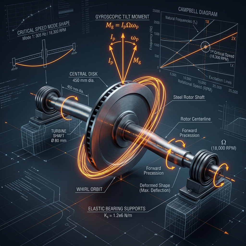
A key distinction in rotor dynamics is the difference between spin and whirl. Spin refers to the rotation of the shaft about its own geometric axis, whereas whirl (or precession) is the orbital motion of the shaft centerline about the line of bearing centers. When a rotor system is brought up to speed, it inevitably encounters resonant conditions, or critical speeds, where the spin speed coincides with one of the natural frequencies of the system's lateral vibrations. Operating a flexible shaft near these critical speeds without sufficient damping leads to catastrophic failure due to uncontrolled vibration amplitudes.

Furthermore, high-speed operation introduces gyroscopic coupling. As the rotor deforms elastically, the disk tilts relative to the rotation axis, generating gyroscopic moments that couple the orthogonal planes of motion (horizontal and vertical). This coupling splits each natural frequency into a forward whirl mode (which increases with spin speed due to gyroscopic stiffening) and a backward whirl mode (which decreases with spin speed due to gyroscopic softening). This article presents a comprehensive study of these phenomena, beginning with the fundamental Jeffcott rotor model, advancing through the rigorous derivation of gyroscopic equations of motion, and examining fluid-film bearing instabilities such as oil whirl and oil whip.

2. The Classical Jeffcott Rotor Model

The Jeffcott rotor model, first analyzed by Henry Jeffcott in 1919, is the foundational building block of rotor dynamics. It consists of a single, rigid, symmetric disk of mass $ m $ mounted at the mid-span of a flexible, massless shaft of bending stiffness $ k $. The shaft is supported at both ends by rigid, frictionless bearings. In this symmetric configuration, the translational motion of the disk is uncoupled from its angular (tilting) motion.

Let $ O-xyz $ be a fixed Cartesian coordinate system where the $ z $-axis coincides with the line of bearing centers. Let the coordinates of the geometric center of the shaft at the disk location be $ C(x, y) $. The center of mass of the disk, $ G $, is offset from $ C $ by a small eccentricity distance $ e $ (mass unbalance) due to manufacturing tolerances or material inhomogeneities. If the shaft spins at a constant angular speed $ \Omega $, the angular orientation of the vector $ \vec{CG} $ relative to the $ x $-axis is given by $ \Omega t $.

The coordinates of the center of mass $ G(x_G, y_G) $ are:

$$ x_G = x + e \cos(\Omega t) $$

$$ y_G = y + e \sin(\Omega t) $$

Applying Newton's second law to the motion of the disk center of mass, and assuming a viscous damping coefficient $ c $ acting on the shaft center, the equations of motion in the $ x $ and $ y $ directions are:

$$ m \ddot{x}_G + c \dot{x} + k x = 0 \implies m \ddot{x} + c \dot{x} + k x = m e \Omega^2 \cos(\Omega t) $$

$$ m \ddot{y}_G + c \dot{y} + k y = 0 \implies m \ddot{y} + c \dot{y} + k y = m e \Omega^2 \sin(\Omega t) $$

To solve these coupled equations, we introduce the complex coordinate $ s = x + i y $. Multiplying the $ y $-equation by $ i $ and adding it to the $ x $-equation yields:

$$ m \ddot{s} + c \dot{s} + k s = m e \Omega^2 e^{i \Omega t} $$

We assume a steady-state synchronous response of the form $ s(t) = S e^{i \Omega t} $, where $ S $ is the complex amplitude of the whirl orbit. Substituting this trial solution and dividing by $ e^{i \Omega t} $ gives:

$$ \left( -m \Omega^2 + i c \Omega + k \right) S = m e \Omega^2 $$

Introducing the undamped natural frequency $ \omega_n = \sqrt{k/m} $, the damping ratio $ \zeta = c / (2 \sqrt{km}) $, and the frequency ratio $ \beta = \Omega / \omega_n $, we can express $ S $ as:

$$ S = e \frac{\beta^2}{(1 - \beta^2) + i (2 \zeta \beta)} = |S| e^{-i \phi} $$

The magnitude of the deflection normalized by the eccentricity, and the phase lag $ \phi $ between the displacement vector $ \vec{OC} $ and the unbalance vector $ \vec{CG} $ are:

$$ \frac{|S|}{e} = \frac{\beta^2}{\sqrt{(1 - \beta^2)^2 + (2 \zeta \beta)^2}} $$

$$ \phi = \tan^{-1}\left( \frac{2 \zeta \beta}{1 - \beta^2} \right) $$

This derivation reveals three critical regimes of rotor behavior:

Sub-critical region ($ \beta \ll 1 $): The phase lag $ \phi \approx 0 $, meaning the heavy spot of the rotor points in the direction of shaft deflection. The vibration amplitude is small and proportional to $ \Omega^2 $.
Resonant region ($ \beta \approx 1 $): The phase lag passes through $ 90^\circ $ ($ \pi/2 $ rad). The deflection amplitude is limited only by the damping: $ |S|_{max} \approx e / (2 \zeta) $. This is the critical speed, where operation is highly dangerous.
Super-critical region ($ \beta \gg 1 $): The phase lag approaches $ 180^\circ $ ($ \pi $ rad), and the amplitude ratio $ |S|/e \to 1 $. Physically, the shaft center deflects by exactly $ -e $, meaning the center of mass $ G $ aligns perfectly with the bearing axis of rotation $ O $. This phenomenon is known as self-centering or automatic balancing, and it allows high-speed turbines to operate stably far above their critical speeds.

Animation: Whirling Shaft Orbit and Phase Relationship

3. Rigorous Derivation of Equations of Motion with Gyroscopic Coupling

In general turbomachinery, the disk is rarely located at the exact mid-span, or the shaft supports are not perfectly symmetric. When the disk is located off-center, the shaft undergoes bending that induces both translational deflections $ x, y $ and angular tilts $ \theta_x, \theta_y $ (rotations about the $ x $ and $ y $ axes, representing pitch and yaw). The spinning disk, when tilted, generates a gyroscopic torque that couples the lateral vibrations in the two orthogonal planes.

Let us derive the equations of motion for a tilted, spinning disk of mass $ m $, polar moment of inertia $ I_p $, and transverse moment of inertia $ I_t $. We define a stationary coordinate system $ O-xyz $ and a body-fixed rotating coordinate system attached to the disk.

To specify the orientation of the disk, we use Euler-like rotations. Starting from the stationary frame, we apply a rotation $ \theta_y $ about the $ y $-axis, followed by a rotation $ \theta_x $ about the new $ x $-axis, and finally a rotation $ \psi $ about the disk's spin axis (with spin speed $ \dot{\psi} = \Omega $). Assuming the angular deflections $ \theta_x $ and $ \theta_y $ are small, the components of the angular velocity vector $ \vec{\omega} $ in the body-fixed axes can be approximated as:

$$ \omega_X \approx \dot{\theta}_x - \Omega \theta_y $$

$$ \omega_Y \approx \dot{\theta}_y + \Omega \theta_x $$

$$ \omega_Z \approx \Omega + \dot{\theta}_x \theta_y \approx \Omega $$

The total kinetic energy $ T $ of the disk is the sum of its translational and rotational kinetic energy:

$$ T = T_{trans} + T_{rot} = \frac{1}{2} m (\dot{x}^2 + \dot{y}^2) + \frac{1}{2} I_t (\omega_X^2 + \omega_Y^2) + \frac{1}{2} I_p \omega_Z^2 $$

Substituting the angular velocity approximations into the kinetic energy expression yields:

$$ T = \frac{1}{2} m (\dot{x}^2 + \dot{y}^2) + \frac{1}{2} I_t \left( (\dot{\theta}_x - \Omega \theta_y)^2 + (\dot{\theta}_y + \Omega \theta_x)^2 \right) + \frac{1}{2} I_p (\Omega + \dot{\theta}_y \theta_x)^2 $$

Expanding this expression and retaining terms up to the second order in coordinates and velocities for a constant spin speed $ \Omega $:

$$ T \approx \frac{1}{2} m (\dot{x}^2 + \dot{y}^2) + \frac{1}{2} I_t (\dot{\theta}_x^2 + \dot{\theta}_y^2) + I_t \Omega (\dot{\theta}_y \theta_x - \dot{\theta}_x \theta_y) + \frac{1}{2} I_p (\Omega^2 + 2 \Omega \dot{\theta}_y \theta_x) $$

Wait, let us simplify the rotational terms using the standard Lagrange equation. The generalized coordinate vector is chosen as $ q = [x, y, \theta_x, \theta_y]^T $. The potential energy $ V $ stored in the elastic shaft is:

$$ V = \frac{1}{2} q^T K q $$

where $ K $ is the symmetric stiffness matrix of the shaft. Let us apply Lagrange's equations of motion:

$$ \frac{d}{dt}\left( \frac{\partial T}{\partial \dot{q}_j} \right) - \frac{\partial T}{\partial q_j} + \frac{\partial V}{\partial q_j} = Q_j $$

Let us calculate the derivatives for the rotational coordinates $ \theta_x $ and $ \theta_y $:

For $ q_3 = \theta_x $:

$$ \frac{\partial T}{\partial \dot{\theta}_x} = I_t \dot{\theta}_x \implies \frac{d}{dt}\left( \frac{\partial T}{\partial \dot{\theta}_x} \right) = I_t \ddot{\theta}_x $$

$$ \frac{\partial T}{\partial \theta_x} = I_p \Omega \dot{\theta}_y $$

Thus, the equation for $ \theta_x $ becomes:

$$ I_t \ddot{\theta}_x - I_p \Omega \dot{\theta}_y + \frac{\partial V}{\partial \theta_x} = M_x $$

For $ q_4 = \theta_y $:

$$ \frac{\partial T}{\partial \dot{\theta}_y} = I_t \dot{\theta}_y + I_p \Omega \theta_x \implies \frac{d}{dt}\left( \frac{\partial T}{\partial \dot{\theta}_y} \right) = I_t \ddot{\theta}_y + I_p \Omega \dot{\theta}_x $$

$$ \frac{\partial T}{\partial \theta_y} = 0 $$

Thus, the equation for $ \theta_y $ becomes:

$$ I_t \ddot{\theta}_y + I_p \Omega \dot{\theta}_x + \frac{\partial V}{\partial \theta_y} = M_y $$

Writing these equations together with the translational equations of motion in matrix form gives:

$$ M \ddot{q} + G \dot{q} + K q = f(t) $$

where the mass matrix $ M $ and the gyroscopic coupling matrix $ G $ are defined as:

$$ M = \begin{bmatrix} m & 0 & 0 & 0 \\ 0 & m & 0 & 0 \\ 0 & 0 & I_t & 0 \\ 0 & 0 & 0 & I_t \end{bmatrix}, \quad G = \begin{bmatrix} 0 & 0 & 0 & 0 \\ 0 & 0 & 0 & 0 \\ 0 & 0 & 0 & -I_p \Omega \\ 0 & 0 & I_p \Omega & 0 \end{bmatrix} $$

The matrix $ G $ is skew-symmetric ($ G^T = -G $), which is a mathematical representation of gyroscopic conservation of energy: gyroscopic forces act perpendicular to the velocity vector and do no work on the system ($ \dot{q}^T G \dot{q} = 0 $). However, they physically couple the pitch and yaw vibrations, leading to frequency splitting.

Animation: Gyroscopic Precession and Vector Interactions

4. Critical Speeds and the Campbell Diagram

To analyze the stability and natural frequencies of the gyroscopic system, we perform an eigenvalue analysis of the homogeneous equation:

$$ M \ddot{q} + G(\Omega) \dot{q} + K q = 0 $$

Assuming a harmonic response of the form $ q = \vec{u} e^{i \omega t} $, where $ \omega $ is the natural frequency, we obtain the quadratic eigenvalue problem:

$$ \left( -\omega^2 M + i \omega G(\Omega) + K \right) \vec{u} = 0 $$

Because $ G(\Omega) $ is proportional to the spin speed $ \Omega $, the natural frequencies $ \omega $ are functions of $ \Omega $. At $ \Omega = 0 $, the gyroscopic matrix vanishes, and the system has double roots (two orthogonal modes for each natural frequency). As $ \Omega $ increases, the gyroscopic term splits each rest natural frequency into two distinct branches:

Forward Whirl (FW): The precession direction is the same as the shaft rotation. The natural frequency of the forward whirl increases with speed (gyroscopic stiffening).
Backward Whirl (BW): The precession direction is opposite to the shaft rotation. The natural frequency of the backward whirl decreases with speed (gyroscopic softening).

This splitting behavior is visually mapped on a **Campbell Diagram** (natural frequencies $ \omega $ plotted against spin speed $ \Omega $). The diagram also contains excitation lines, the most important being the synchronous excitation line $ \omega = \Omega $ (1x line), which corresponds to the excitation frequency of a rotor with mass unbalance.

The intersections of the natural frequency curves with the 1x excitation line define the **synchronous critical speeds**. In symmetric systems, synchronous mass unbalance only excites the forward whirl modes. Thus, the forward critical speeds represent the actual operational critical speeds where large resonant vibrations occur. The backward critical speeds are generally not excited by unbalance but can be excited by support asymmetry, friction, or internal damping.

5. Unbalance Response of Gyroscopic Rotors

To evaluate the vibration levels of a turbomachine, we must calculate the steady-state response to synchronous unbalance. In the presence of mass eccentricity $ e $, the unbalance force acts at the spin speed $ \Omega $. The force vector $ f(t) $ is:

$$ f(t) = \begin{bmatrix} m e \Omega^2 \cos(\Omega t) \\ m e \Omega^2 \sin(\Omega t) \\ 0 \\ 0 \end{bmatrix} = \operatorname{Re}\left( \begin{bmatrix} m e \Omega^2 \\ -i m e \Omega^2 \\ 0 \\ 0 \end{bmatrix} e^{i \Omega t} \right) $$

By using the complex coordinates $ s = x + i y $ and $ \psi = \theta_y - i \theta_x $, the equations of motion with damping can be simplified. Assuming viscous damping $ c_s $ on translational motion and $ c_\psi $ on angular motion, the coupled equations of motion in complex form are:

$$ m \ddot{s} + c_s \dot{s} + k_{11} s + k_{12} \psi = m e \Omega^2 e^{i \Omega t} $$

$$ I_t \ddot{\psi} - i I_p \Omega \dot{\psi} + c_\psi \dot{\psi} + k_{12} s + k_{22} \psi = 0 $$

For steady-state synchronous whirl, we assume $ s(t) = S e^{i \Omega t} $ and $ \psi(t) = \Psi e^{i \Omega t} $. Substituting these into the equations yields a complex linear system for the amplitudes:

$$ \begin{bmatrix} k_{11} - m \Omega^2 + i c_s \Omega & k_{12} \\ k_{12} & k_{22} + (I_p - I_t)\Omega^2 + i c_\psi \Omega \end{bmatrix} \begin{bmatrix} S \\ \Psi \end{bmatrix} = \begin{bmatrix} m e \Omega^2 \\ 0 \end{bmatrix} $$

Solving this linear system determines the amplitude and phase of the translation orbit $ S $ and rotational tilt orbit $ \Psi $. For a symmetric system with symmetric bearings, the orbits are circular. If the support stiffness is asymmetric (e.g., $ k_{xx} \neq k_{yy} $), the orbits become elliptical, containing both forward and backward whirl components.

6. Fluid-Film Bearing Instabilities: Oil Whirl and Oil Whip

High-speed turbines are commonly supported by hydrodynamic fluid-film journal bearings due to their high load-carrying capacity, long lifespan, and excellent vibration damping. However, fluid-film bearings introduce a serious vibration threat: self-excited hydrodynamic instabilities known as **oil whirl** and **oil whip**.

In a journal bearing, the rotation of the journal drags lubricating oil into the wedge-shaped clearance space between the journal and the bearing sleeve. This builds hydrodynamic pressure that supports the radial load. Under dynamic conditions, the force generated by the fluid film can be linearized about the equilibrium position using eight bearing coefficients:

$$ \begin{bmatrix} F_x \\ F_y \end{bmatrix} = - \begin{bmatrix} k_{xx} & k_{xy} \\ k_{yx} & k_{yy} \end{bmatrix} \begin{bmatrix} x \\ y \end{bmatrix} - \begin{bmatrix} c_{xx} & c_{xy} \\ c_{yx} & c_{yy} \end{bmatrix} \begin{bmatrix} \dot{x} \\ \dot{y} \end{bmatrix} $$

The off-diagonal terms $ k_{xy} $ and $ k_{yx} $ are the **cross-coupled stiffness coefficients**. For a concentric journal, $ k_{xy} \approx -k_{yx} $. These coefficients represent a tangential force that acts perpendicular to the radial displacement of the journal. This tangential force acts as a non-conservative source of energy, dragging the journal into a circular precession (whirl).

Oil Whirl: Because the oil film is dragged by the rotating journal, the average velocity of the oil in the clearance is approximately $ 45\% $ to $ 48\% $ of the journal's surface speed. If the system damping is insufficient to dissipate the energy inputted by the cross-coupled stiffness, the journal begins to whirl at a frequency of:

$$ \omega_{whirl} \approx 0.45 \Omega \text{ to } 0.48 \Omega $$

Oil whirl is sub-synchronous, and its frequency tracks the shaft spin speed $ \Omega $ linearly as the turbine accelerates.

Oil Whip: As the spin speed $ \Omega $ increases, the oil whirl frequency also increases. When $ \omega_{whirl} $ approaches the first critical bending speed of the rotor ($ \omega_{n1} $), the whirl frequency "locks in" to the natural frequency. Any further increase in the spin speed $ \Omega $ does not increase the whirl frequency; instead, it remains fixed at $ \omega_{n1} $. This phenomenon is called **oil whip**. During oil whip, the damping of the oil film is completely overwhelmed, and the rotor undergoes violent, high-amplitude vibrations that can destroy the bearings and shaft within seconds.

Animation: Oil Whirl and Whip Instability in Journal Bearings

Comparison of Bearing and Damper Technologies

Bearing Type	Cross-Coupled Stiffness	Damping Capacity	Stability Level	Primary Instability Limit	Common Applications
Cylindrical Journal	Very High	Moderate	Low	Oil whirl at $ \Omega \approx 2\omega_{n1} $	Low-speed turbines, heavy gearboxes
Multi-Lobe Bearings	Moderate	Good	Moderate	Whirl at higher speed threshold	Turbochargers, medium compressors
Tilting-Pad (TPJB)	Negligible (Zero)	Excellent	Very High	Thermomechanical pad deformation	High-speed compressors, steam turbines
Squeeze Film Damper	Zero (Non-rotating)	Very High	N/A (Used with rolling elements)	Oil film cavitation	Aircraft gas turbines, turbojet engines
Gas Foil Bearings	Low	Low	High	Sub-harmonic foil whirl	Microturbines, air cycle machines

7. Schematic of the Jeffcott Rotor with Gyroscopic Terms

The interactive SVG diagram below illustrates the coordinates, forces, and moments acting on an off-center Jeffcott rotor. The elastic shaft is deflected vertically, causing the disk to tilt by $ \theta_y $ relative to the nominal vertical axis. The spin velocity $ \Omega $ and the rate of tilt change generate a gyroscopic moment $ M_g = -I_p \Omega \dot{\theta}_x $ that couples the lateral vibration planes.

8. Worked Numerical Example

To illustrate the application of these rotor dynamics equations, we solve a detailed exam-style problem for a single-disk rotor with gyroscopic coupling.

Problem Statement

A steel turbine rotor consists of a single, thin, rigid disk mounted on a solid circular shaft of length $ L = 1.0 \text{ m} $ and diameter $ d = 50 \text{ mm} $. The shaft is simply supported at both ends by rigid bearings. The disk is located off-center at a distance $ a = 0.3 \text{ m} $ from the left support (meaning $ b = 0.7 \text{ m} $ from the right support). The rotor properties are:

Disk mass, $ m = 20.0 \text{ kg} $
Polar moment of inertia, $ I_p = 0.25 \text{ kg}\cdot\text{m}^2 $
Transverse moment of inertia, $ I_t = 0.125 \text{ kg}\cdot\text{m}^2 $
Shaft Modulus of Elasticity, $ E = 200 \text{ GPa} = 2 \times 10^{11} \text{ N/m}^2 $
Disk mass eccentricity, $ e = 15 \ \mu\text{m} = 1.5 \times 10^{-5} \text{ m} $

Tasks:

Determine the bending stiffness coefficients ($ k_{11}, k_{12}, k_{22} $) of the shaft.
Calculate the natural frequencies of the system at rest ($ \Omega = 0 $).
Derive the frequency equations and compute the synchronous forward and backward critical speeds.
Calculate the steady-state unbalance response (translational amplitude $ S $ and rotational tilt amplitude $ \Psi $) at an operating speed of $ 3000 \text{ RPM} $ under two cases: (a) without damping, and (b) with damping ($ c_s = 150 \text{ N}\cdot\text{s/m} $ and $ c_\psi = 1.5 \text{ N}\cdot\text{s}\cdot\text{m/rad} $).

Step 1: Calculate Bending Stiffness Coefficients

First, we calculate the area moment of inertia $ I_s $ of the shaft's circular cross-section:

$$ I_s = \frac{\pi d^4}{64} = \frac{\pi (0.05 \text{ m})^4}{64} \approx 3.067962 \times 10^{-7} \text{ m}^4 $$

The bending stiffness parameter $ EI_s $ is:

$$ EI_s = (2 \times 10^{11} \text{ N/m}^2) \times (3.067962 \times 10^{-7} \text{ m}^4) = 61,359.23 \text{ N}\cdot\text{m}^2 $$

Using elastic beam deflection theory for a simply supported beam loaded at $ z = a $, the translational and rotational influence coefficients (flexibility coefficients) at the disk location are:

$$ \alpha_{11} = \frac{a^2 b^2}{3 E I_s L} = \frac{(0.3)^2 (0.7)^2}{3 \times 61,359.23 \times 1.0} = 2.395728 \times 10^{-7} \text{ m/N} $$

$$ \alpha_{12} = \alpha_{21} = \frac{a b (b - a)}{3 E I_s L} = \frac{0.3 \times 0.7 \times (0.7 - 0.3)}{3 \times 61,359.23 \times 1.0} = 4.563291 \times 10^{-7} \text{ rad/N} $$

$$ \alpha_{22} = \frac{L^2 - 3 a b}{3 E I_s L} = \frac{1.0^2 - 3 \times 0.3 \times 0.7}{3 \times 61,359.23 \times 1.0} = 2.010021 \times 10^{-6} \text{ rad/(N}\cdot\text{m)} $$

The flexibility matrix $ [\alpha] $ is defined as:

$$ [\alpha] = \begin{bmatrix} 2.395728 \times 10^{-7} & 4.563291 \times 10^{-7} \\ 4.563291 \times 10^{-7} & 2.010021 \times 10^{-6} \end{bmatrix} $$

The stiffness matrix $ [k] $ is the inverse of the flexibility matrix:

$$ [k] = [\alpha]^{-1} = \frac{1}{\det([\alpha])} \begin{bmatrix} \alpha_{22} & -\alpha_{12} \\ -\alpha_{12} & \alpha_{11} \end{bmatrix} $$

Calculating the determinant:

$$ \det([\alpha]) = (2.395728 \times 10^{-7})(2.010021 \times 10^{-6}) - (4.563291 \times 10^{-7})^2 = 2.733054 \times 10^{-13} $$

Inverting the matrix gives the stiffness coefficients:

$$ k_{11} = \frac{2.010021 \times 10^{-6}}{2.733054 \times 10^{-13}} = 7,354,582 \text{ N/m} = 7.3546 \text{ MN/m} $$

$$ k_{12} = k_{21} = \frac{-4.563291 \times 10^{-7}}{2.733054 \times 10^{-13}} = -1,669,709 \text{ N/rad} = -1.6697 \text{ MN/rad} $$

$$ k_{22} = \frac{2.395728 \times 10^{-7}}{2.733054 \times 10^{-13}} = 876,585 \text{ N}\cdot\text{m/rad} = 0.8766 \text{ MN}\cdot\text{m/rad} $$

Step 2: Calculate Natural Frequencies at Rest ($ \Omega = 0 $)

At rest, the translational and rotational coordinates are coupled, but there are no gyroscopic forces. The equations of motion for a single lateral plane (e.g., $ x - \theta_y $) are:

$$ \begin{bmatrix} m & 0 \\ 0 & I_t \end{bmatrix} \begin{bmatrix} \ddot{x} \\ \ddot{\theta}_y \end{bmatrix} + \begin{bmatrix} k_{11} & k_{12} \\ k_{12} & k_{22} \end{bmatrix} \begin{bmatrix} x \\ \theta_y \end{bmatrix} = \begin{bmatrix} 0 \\ 0 \end{bmatrix} $$

Setting the determinant of $ [k] - \omega^2 [M] $ to zero gives the characteristic equation:

$$ \det \begin{bmatrix} k_{11} - m \omega^2 & k_{12} \\ k_{12} & k_{22} - I_t \omega^2 \end{bmatrix} = 0 \implies m I_t \omega^4 - (m k_{22} + I_t k_{11}) \omega^2 + (k_{11} k_{22} - k_{12}^2) = 0 $$

Substituting the numerical values into the coefficients:

$ m I_t = 20.0 \times 0.125 = 2.5 \text{ kg}^2\cdot\text{m}^2 $
$ m k_{22} + I_t k_{11} = 20.0 \times 876,585 + 0.125 \times 7,354,582 = 17,531,700 + 919,322.75 = 18,451,022.75 \text{ kg}\cdot\text{N}\cdot\text{m} $
$ \det(k) = k_{11} k_{22} - k_{12}^2 = 7,354,582 \times 876,585 - (-1,669,709)^2 = 3.65899 \times 10^{12} \text{ N}^2/\text{rad} $

The quadratic equation in $ \omega^2 $ is:

$$ 2.5 \omega^4 - 18,451,022.75 \omega^2 + 3.65899 \times 10^{12} = 0 $$

Solving this quadratic yields the roots:

$$ \omega_{n1}^2 = 203,942.34 \implies \omega_{n1} = 451.60 \text{ rad/s} \quad (71.87 \text{ Hz, or } 4312.5 \text{ RPM}) $$

$$ \omega_{n2}^2 = 7,176,466.76 \implies \omega_{n2} = 2678.89 \text{ rad/s} \quad (426.36 \text{ Hz, or } 25581.3 \text{ RPM}) $$

Step 3: Calculate Synchronous Critical Speeds

Under synchronous whirl ($ \omega = \Omega $), we solve for the spin speeds where resonance occurs.

Case A: Forward Whirl (FW): The frequency equation for synchronous forward whirl is derived by substituting $ \omega = \Omega $ into the complex equations, giving:

$$ \det \begin{bmatrix} k_{11} - m \Omega^2 & k_{12} \\ k_{12} & k_{22} + (I_p - I_t) \Omega^2 \end{bmatrix} = 0 $$

Expanding this determinant yields:

$$ -m (I_p - I_t) \Omega^4 + [ k_{11}(I_p - I_t) - m k_{22} ] \Omega^2 + (k_{11} k_{22} - k_{12}^2) = 0 $$

Substituting the parameters ($ I_p - I_t = 0.25 - 0.125 = 0.125 \text{ kg}\cdot\text{m}^2 $):

$ A_{fw} = -m(I_p - I_t) = -20.0 \times 0.125 = -2.5 $
$ B_{fw} = 7,354,582 \times 0.125 - 20.0 \times 876,585 = 919,322.75 - 17,531,700 = -16,612,377.25 $
$ C_{fw} = 3.65899 \times 10^{12} $

The quadratic equation in $ \Omega^2 $ is:

$$ -2.5 \Omega^4 - 16,612,377.25 \Omega^2 + 3.65899 \times 10^{12} = 0 $$

Solving this equation, we get the roots for $ \Omega^2 $:

$$ \Omega_{cr,F1}^2 = 213,401.0 \implies \Omega_{cr,F1} = 461.95 \text{ rad/s} \quad (4411.33 \text{ RPM}) $$

$$ \Omega_{cr,F2}^2 = -6,858,351.9 \quad (\text{No physical real root}) $$

Because $ I_p > I_t $, the gyroscopic stiffening is so strong that the second forward whirl mode is shifted upward faster than the spin speed increases. Consequently, the synchronous unbalance line $ \omega = \Omega $ never intersects the second forward frequency branch, meaning **there is only one physical critical speed in forward whirl**.

Case B: Backward Whirl (BW): The frequency equation for synchronous backward whirl is derived by substituting $ \omega = -\Omega $ into the complex equations, giving:

$$ \det \begin{bmatrix} k_{11} - m \Omega^2 & k_{12} \\ k_{12} & k_{22} - (I_p + I_t) \Omega^2 \end{bmatrix} = 0 $$

Expanding this determinant yields:

$$ m (I_p + I_t) \Omega^4 - [ k_{11}(I_p + I_t) + m k_{22} ] \Omega^2 + (k_{11} k_{22} - k_{12}^2) = 0 $$

Substituting the parameters ($ I_p + I_t = 0.25 + 0.125 = 0.375 \text{ kg}\cdot\text{m}^2 $):

$ A_{bw} = m(I_p + I_t) = 20.0 \times 0.375 = 7.5 $
$ B_{bw} = -(7,354,582 \times 0.375 + 20.0 \times 876,585) = -(2,757,968.25 + 17,531,700) = -20,289,668.25 $
$ C_{bw} = 3.65899 \times 10^{12} $

The quadratic equation in $ \Omega^2 $ is:

$$ 7.5 \Omega^4 - 20,289,668.25 \Omega^2 + 3.65899 \times 10^{12} = 0 $$

Solving this yields two positive roots for $ \Omega^2 $:

$$ \Omega_{cr,B1}^2 = 194,290.1 \implies \Omega_{cr,B1} = 440.78 \text{ rad/s} \quad (4209.17 \text{ RPM}) $$

$$ \Omega_{cr,B2}^2 = 2,510,999.0 \implies \Omega_{cr,B2} = 1584.61 \text{ rad/s} \quad (15132.0 \text{ RPM}) $$

In backward whirl, the gyroscopic forces act as a softening effect, lowering the natural frequencies and allowing both modes to be crossed.

Step 4: Unbalance Response at 3000 RPM ($ \Omega = 314.1593 \text{ rad/s} $)

At $ 3000 \text{ RPM} $ (which is below the first critical speed), the unbalance force magnitude is:

$$ m e \Omega^2 = 20.0 \times (1.5 \times 10^{-5}) \times (314.1593)^2 = 29.6088 \text{ N} $$

Case A: Undamped Response: We solve:

$$ S = \frac{m e \Omega^2}{k_{11} - m \Omega^2 - \frac{k_{12}^2}{k_{22} + (I_p - I_t) \Omega^2}} $$

Calculating the terms:

$ m \Omega^2 = 20.0 \times (314.1593)^2 = 1,973,921.2 \text{ N/m} $
$ (I_p - I_t) \Omega^2 = 0.125 \times (314.1593)^2 = 12,337.0 \text{ N}\cdot\text{m/rad} $
$ k_{22} + (I_p - I_t) \Omega^2 = 876,585 + 12,337 = 888,922 \text{ N}\cdot\text{m/rad} $
$ \text{denom\_term} = \frac{k_{12}^2}{888,922} = \frac{(-1,669,709)^2}{888,922} = 3,136,186 \text{ N/m} $
$ \text{denom} = k_{11} - m \Omega^2 - \text{denom\_term} = 7,354,582 - 1,973,921.2 - 3,136,186 = 2,244,474.8 \text{ N/m} $

Solving for translational amplitude $ S $:

$$ S = \frac{29.6088}{2,244,474.8} = 1.31928 \times 10^{-5} \text{ m} = 13.19 \ \mu\text{m} $$

Solving for rotational tilt amplitude $ \Psi $:

$$ \Psi = -\frac{k_{12} S}{k_{22} + (I_p - I_t) \Omega^2} = -\frac{(-1,669,709)(1.31928 \times 10^{-5})}{888,922} = 2.4780 \times 10^{-5} \text{ rad} \quad (0.00142^\circ) $$

Case B: Damped Response ($ c_s = 150 \text{ N}\cdot\text{s/m} $, $ c_\psi = 1.5 \text{ N}\cdot\text{s}\cdot\text{m/rad} $):

We solve the complex system:

Substituting values:

$ c_s \Omega = 150 \times 314.1593 = 47,123.9 \text{ N/m} $
$ c_\psi \Omega = 1.5 \times 314.1593 = 471.24 \text{ N}\cdot\text{m/rad} $

$$ \begin{bmatrix} 5,380,660.8 + 47,123.9 i & -1,669,709 \\ -1,669,709 & 888,922 + 471.24 i \end{bmatrix} \begin{bmatrix} S \\ \Psi \end{bmatrix} = \begin{bmatrix} 29.6088 \\ 0 \end{bmatrix} $$

Solving this system yields:

$$ S = (1.3187 - 0.0287 i) \times 10^{-5} \text{ m} \implies |S| = 1.3190 \times 10^{-5} \text{ m} = 13.19 \ \mu\text{m}, \quad \text{Phase } \phi_s = -1.25^\circ $$

$$ \Psi = (2.4768 - 0.0552 i) \times 10^{-5} \text{ rad} \implies |\Psi| = 2.4775 \times 10^{-5} \text{ rad} \quad (0.00142^\circ), \quad \text{Phase } \phi_\psi = -1.28^\circ $$

The damping introduces a small phase lag in the precession and slightly reduces the amplitudes of both the translational deflection and the angular tilt orbits.

Rotor Dynamics & Gyroscopic Stability in High-Speed Turbines

Rotor Dynamics & Gyroscopic Stability in High-Speed Turbines

1. Introduction to Rotor Dynamics in High-Speed Turbomachinery

2. The Classical Jeffcott Rotor Model

Animation: Whirling Shaft Orbit and Phase Relationship

3. Rigorous Derivation of Equations of Motion with Gyroscopic Coupling

Animation: Gyroscopic Precession and Vector Interactions

4. Critical Speeds and the Campbell Diagram

5. Unbalance Response of Gyroscopic Rotors

6. Fluid-Film Bearing Instabilities: Oil Whirl and Oil Whip

Animation: Oil Whirl and Whip Instability in Journal Bearings

Comparison of Bearing and Damper Technologies

7. Schematic of the Jeffcott Rotor with Gyroscopic Terms

8. Worked Numerical Example

Problem Statement

Tasks:

Step 1: Calculate Bending Stiffness Coefficients

Step 2: Calculate Natural Frequencies at Rest (\( \Omega = 0 \))

Step 3: Calculate Synchronous Critical Speeds

Step 4: Unbalance Response at 3000 RPM (\( \Omega = 314.1593 \text{ rad/s} \))