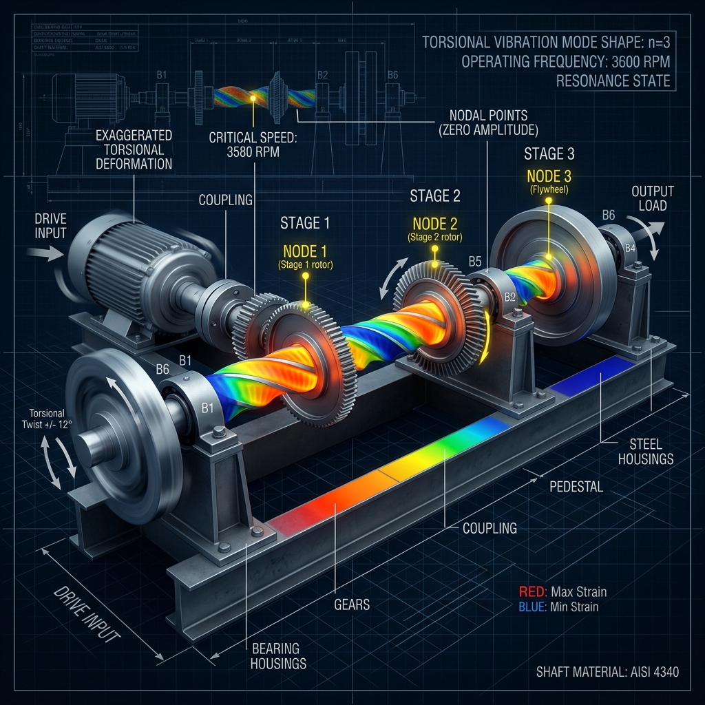
Torsional Vibration and Critical Speed Analysis of Multistage Power Transmission Shafts

Section 1: Introduction and Mechanical Fundamentals of Shaft Vibrations

1.1 Overview of Rotor-Dynamic Nomenclature and Reference Coordinates

The design, operation, and maintenance of high-performance turbomachinery—including steam and gas turbines, multistage centrifugal compressors, generators, and marine propulsion systems—require a rigorous understanding of rotor-dynamics. In these high-power, high-speed machines, the rotating shaft acts as the primary transmission path for mechanical energy. As operating speeds increase and structural weight is minimized to enhance thermodynamic efficiency, shafts are subjected to severe dynamic loads that can drive the system into destructive resonant states.

To establish a rigorous mathematical treatment of these vibrations, we must define the coordinate systems and mechanical properties that govern the rotor-dynamic behavior. We establish a fixed inertial coordinate frame $\{O; X, Y, Z\}$ and a rotating coordinate frame $\{o; x, y, z\}$ that rotates about the nominal shaft axis $Z$ at an angular velocity $\Omega$. The displacement of any cross-section of the shaft is defined by translation coordinates $(X, Y)$ representing lateral deflection, axial coordinate $Z$, tilt angles $(\theta_x, \theta_y)$ representing the slope of the shaft centerline due to bending, and the torsional twist angle $\theta(z, t)$ representing the rotation of the cross-section relative to the nominal rotation angle $\Omega t$. The mechanical variables and parameters used throughout this monograph are defined in the nomenclature table below.

Table 1.1: Physical Nomenclature and SI Units for Shaft Vibrations

Symbol	Parameter / Physical Property Description	SI Units
$\theta(z, t)$	Torsional angular displacement (twist angle)	$\text{rad}$
$T(z, t)$	Internal torsional torque acting on the cross-section	$\text{N}\cdot\text{m}$
$G$	Shear modulus of rigidity of the shaft material	$\text{Pa} \ (\text{N/m}^2)$
$\rho$	Mass density of the shaft material	$\text{kg/m}^3$
$J(z)$	Polar area moment of inertia of the shaft cross-section	$\text{m}^4$
$I_p(z)$	Polar mass moment of inertia per unit length ($I_p = \rho J$)	$\text{kg}\cdot\text{m}$
$c$	Torsional wave propagation speed ($c = \sqrt{G/\rho}$)	$\text{m/s}$
$\omega$	Dynamic oscillation frequency (natural frequency or excitation frequency)	$\text{rad/s}$
$\Omega$	Nominal rotational speed of the shaft	$\text{rad/s}$
$k_t$	Equivalent torsional stiffness of a shaft segment	$\text{N}\cdot\text{m/rad}$
$J_i$	Mass moment of inertia of the $i$-th lumped rotor or disc	$\text{kg}\cdot\text{m}^2$
$e$	Mass eccentricity (offset between geometric center and mass center)	$\text{m}$
$f_m$	Gear meshing frequency ($f_m = N \cdot \Omega / (2\pi)$)	$\text{Hz}$
$\mathbf{M}$	Global mass moment of inertia matrix	$\text{kg}\cdot\text{m}^2$
$\mathbf{K}$	Global torsional stiffness matrix	$\text{N}\cdot\text{m/rad}$
$\mathbf{C}$	Global torsional damping matrix	$\text{N}\cdot\text{m}\cdot\text{s/rad}$

1.2 Kinematics and Phenomenology: Lateral vs. Torsional Vibrations

Shaft vibrations are broadly categorized into two fundamental modes: lateral (bending/whirling) vibrations and torsional vibrations. Understanding the physical differences, manifestation symptoms, and kinematic coupling between these modes is essential for accurate diagnostics and structural design.

Lateral vibrations involve the physical displacement of the shaft's geometric centerline perpendicular to its nominal axis of rotation. This motion manifests as a bending deformation of the shaft under dynamic loads, resulting in radial displacements in the $X$- and $Y$-directions. When the shaft rotates, these lateral displacements sweep out a three-dimensional orbit, a phenomenon known as whirling. Lateral vibrations are driven by centrifugal forces arising from mass unbalance, gyroscopic moments, and fluid forces in bearings. Gyroscopic moments couple the translations and tilts in the $X$- and $Y$-planes, causing the natural frequencies to split into forward whirling modes (where the orbit direction matches shaft rotation) and backward whirling modes (orbit direction opposes shaft rotation). Lateral vibrations are easily detected because they transmit large dynamic forces to the stator casing through the bearings, which are captured by casing accelerometers or shaft proximity probes.

In contrast, torsional vibrations involve the angular oscillation of shaft cross-sections relative to each other about the longitudinal axis of rotation. In this mode, the centerline of the shaft remains perfectly straight, and there is no lateral displacement of the shaft centerline. Consequently, torsional vibrations do not generate radial forces at the bearings and do not transmit vibrations to the stationary casing. For this reason, torsional vibrations are often referred to as the "silent killers" of rotating machinery. A turbomachine can operate under high-amplitude torsional resonance with no outward signs of distress—no noise, no casing vibration, and no temperature spikes—until a shaft undergoes sudden, catastrophic shear failure due to torsional fatigue, or gear teeth shear off in the gearbox.

Although lateral and torsional vibrations are often modeled independently for simple systems, they are strongly coupled in complex multistage power transmission shafts through several physical mechanisms:

• Geared Assemblies: In geared systems, the gear mesh force acts along the line of action, which is tangent to the base circles of the mating gears. As a result, any torsional oscillation of the gears alters the contact force, generating a direct radial force that excites lateral vibrations of the shafts. Conversely, lateral displacement of the shafts alters the center-to-center distance of the gears, introducing geometric transmission errors that excite torsional oscillations.
• Mass Eccentricity: For a rotor with mass eccentricity $e$, the center of mass is offset from the geometric center. If the shaft undergoes torsional acceleration $\ddot{\theta}$, the circumferential acceleration of the center of mass generates a lateral force proportional to $m e \ddot{\theta}$. Conversely, lateral acceleration of the shaft center of gravity exerts an inertial torque $m e \ddot{X}$ about the geometric center, coupling the two modes.
• Curved Shaft Geometry: A shaft with an initial geometric bend or thermal bow undergoes cyclic gravity bending under rotation. The resulting asymmetric stiffness in the bending plane causes periodic variations in the required driving torque, exciting torsional oscillations at the rotational frequency ($1\Omega$) and its second harmonic ($2\Omega$).

1.3 Primary Sources of Dynamic Excitation

Dynamic excitation forces in power transmission shafts originate from mechanical manufacturing limitations, joint kinematics, kinematics of power sources, and the nature of the driven load. The three most prevalent sources of excitation are mass unbalance, gear meshing dynamics, and reciprocating engine kinematics.

1.3.1 Mass Unbalance and the Jeffcott Rotor Formulation

Mass unbalance is the most common source of lateral excitation. Even with high-precision balancing, a rotor has a residual eccentricity $e$, where the center of mass $G$ is offset from the geometric center $S$. To model this, we consider the classic Jeffcott rotor model: a single symmetric disc of mass $m$ mounted at the midspan of a massless, flexible shaft of lateral stiffness $k$ and viscous damping $c$.

Let the coordinates of the geometric center $S$ in the fixed inertial frame $\{O; X, Y\}$ be $(X, Y)$, and let the shaft rotate at a constant angular velocity $\omega$. The coordinates of the center of mass $G$ are:

Applying Newton's second law to the motion of the center of mass yields the equations of motion for the rotor:

These decoupled linear differential equations show that the mass unbalance acts as a harmonic excitation force of magnitude $F_0 = m e \omega^2$ that increases quadratically with speed. The steady-state lateral displacement amplitude $A$ of the shaft geometric center is:

where $r = \omega / \omega_n$ is the frequency ratio, $\omega_n = \sqrt{k/m}$ is the lateral natural frequency (critical speed), and $\zeta = c / (2\sqrt{k m})$ is the damping ratio. The phase lag $\phi$ of the response relative to the unbalance force is:

When the rotational speed $\omega$ matches the natural frequency $\omega_n$ ($r = 1$), the system enters resonance. The lateral amplitude is limited only by damping, $A_{\text{res}} = e / (2\zeta)$. At high speeds ($r \gg 1$), the amplitude $A$ approaches $e$, and the phase angle $\phi$ approaches $180^\circ$. This indicates that the geometric center $S$ rotates around the mass center $G$, which remains stationary at the origin $O$, a self-centering phenomenon key to high-speed rotor operation.

1.3.2 Gear Meshing Dynamics and Stiffness Variations

Gearboxes are major sources of high-frequency torsional and lateral vibrations. The gear-mesh interface is characterized by three distinct physical excitation mechanisms:

1. Variable Mesh Stiffness ($k_m(t)$): As gears rotate, the number of teeth in contact alternates periodically (e.g., between single tooth contact and double tooth contact for spur gears). This variation causes the stiffness of the gear mesh to fluctuate periodically at the gear-meshing frequency $f_m = N \cdot \Omega / (2\pi)$, where $N$ is the number of teeth on the gear and $\Omega$ is its angular velocity. The mesh stiffness can be modeled as a Fourier series:

where $k_{m0}$ is the mean mesh stiffness, and $k_{mn}$ represents the harmonic amplitudes at the meshing frequency $\omega_m = 2\pi f_m$. This parametric stiffness variation excites parametric resonance.

2. Transmission Error (TE): Transmission error is defined as the deviation of the actual position of the driven gear from its theoretical position:

TE is caused by manufacturing imperfections (pitch and profile errors) and elastic deformation of the teeth under load. It acts as a displacement excitation at the mesh interface, generating high-frequency torsional vibration.

3. Backlash and Tooth Separation: Backlash is the clearance between mating gear teeth designed to prevent jamming. Under torque reversals or high-amplitude vibrations, the teeth can lose contact. This results in piecewise-linear stiffness behavior, modeled as:

where $b$ is the total backlash and $\delta$ is the relative displacement along the line of action. When teeth separate and re-engage, impact forces occur, exciting high-frequency structural modes.

1.3.3 Reciprocating Engine Excitation

In systems driven by reciprocating internal combustion engines or reciprocating compressors, the crankshaft is subjected to highly non-uniform torque. This excitation consists of gas pressure forces and inertial forces from the reciprocating components.

For a single cylinder, let $P(\alpha)$ be the cylinder pressure at crank angle $\alpha$, $A$ be the piston area, $r$ be the crank radius, $L$ be the connecting rod length, and $\lambda = r/L$. The force acting on the piston is $F_p = P(\alpha) A$. Resolving this force through the slider-crank kinematics yields the gas torque on the crankshaft:

Because cylinder pressure $P(\alpha)$ is periodic over the engine cycle ($4\pi$ radians for a 4-stroke engine, $2\pi$ for a 2-stroke engine), the torque can be expanded as a Fourier series:

where $\omega_e$ is the engine angular velocity. The harmonic orders $n$ are integers ($n = 1, 2, 3, \dots$) for 2-stroke engines, and half-integers and integers ($n = 0.5, 1.0, 1.5, 2.0, \dots$) for 4-stroke engines.

The second excitation source is the inertia of the reciprocating mass $m_{\text{rec}}$ (piston, wrist pin, and small end of the connecting rod). The acceleration of the piston is approximately:

The inertia force $F_{\text{inertia}} = -m_{\text{rec}} a_p$ produces a torque on the crankshaft. By expanding the kinematics, the reciprocating inertia torque is:

This torque is proportional to the square of the engine speed ($\omega_e^2$) and excites the 1st, 2nd, 3rd, and 4th engine harmonics. The sum of these gas and inertia torques across all cylinders yields a highly dynamic excitation spectrum. If any engine harmonic frequency matches a torsional natural frequency of the shaft system, severe resonance can occur.

1.4 Dynamic Impact on Bearings and Couplings

Dynamic shaft displacements and forces degrade the performance of support bearings and flexible couplings, reducing operating life and causing mechanical failures.

1.4.1 Bearing Dynamics and Stability

In heavy turbomachinery, shafts are supported by fluid-film journal bearings. Under dynamic loads, the dynamic behavior of the oil film is modeled by linearized stiffness and damping coefficients that couple the $X$ and $Y$ lateral directions:

The dynamic pressure distribution within the fluid film is governed by the two-dimensional Reynolds equation:

where $h$ is the oil film thickness, $\mu$ is dynamic viscosity, $U$ is surface velocity, and $P$ is pressure. The cross-coupling stiffness coefficients ($k_{xy}$ and $k_{yx}$) represent the lateral force generated perpendicular to the shaft displacement due to hydrodynamic pressure rotation. If these terms are large, they act as a source of energy input to the lateral modes, exciting a self-excited instability known as oil whirl. Oil whirl occurs at a frequency slightly below half of the rotational speed ($\approx 0.48\Omega$). If the shaft speed is increased such that the oil whirl frequency matches the first lateral natural frequency of the rotor, the system enters oil whip. Oil whip is a severe instability where lateral vibration amplitudes grow rapidly, leading to metal-to-metal contact in the bearing and catastrophic failure.

For systems supported by rolling element bearings, lateral and torsional vibrations generate dynamic loads that exceed the static design capacity. Under static and dynamic loads, the rolling element contact is governed by Hertzian contact theory. The relation between contact load $Q$ and elastic deformation $\delta$ is:

where $K_p$ and $K_l$ are the Hertzian contact stiffness constants. According to the Lundberg-Palmgren fatigue theory, the rating life $L_{10}$ of a rolling element bearing is:

where $C$ is the basic dynamic load rating, $P$ is the equivalent dynamic load, and $p$ is the fatigue exponent (3 for ball bearings, $10/3$ for roller bearings). High-amplitude lateral vibrations increase the dynamic load $P$, causing a non-linear reduction in the bearing's fatigue life.

1.4.2 Coupling Dynamics under Misalignment

Couplings are used to connect shaft segments, but they must often operate with some parallel or angular misalignment. When shafts are connected by a universal (Cardan) joint under an angular misalignment angle $\beta$, the kinematic relation between the input angle $\phi$ and output angle $\psi$ is non-linear:

Differentiating this relation with respect to time yields the ratio of output to input angular velocities:

For small misalignment angles $\beta$, we can expand this velocity ratio using a Taylor series approximation:

This expansion shows that a misaligned Cardan joint introduces periodic velocity fluctuations at the second harmonic ($2\phi \approx 2\omega t$) of the rotational speed. Additionally, under a constant resisting load torque $T_{\text{out}}$ on the driven shaft, the torque transmitted back to the driving shaft $T_{\text{in}}$ fluctuates according to:

This torque fluctuation acts as a direct source of torsional excitation. Flexible couplings (e.g., diaphragm, gear, or grid couplings) are designed to provide axial, radial, and torsional compliance to isolate these excitations, but they introduce complex damping behaviors and shift the system's torsional natural frequencies.

Section 2: Mathematical Modeling of Free Torsional Vibrations

2.1 Continuous Modeling: Derivation of the Wave Equation

To model torsional vibrations, we must treat the shaft as a continuous elastic body. We assume the shaft is axisymmetric, isotropic, and obeys Hooke's law, and that plane cross-sections remain plane and rotate as rigid surfaces during deformation.

Consider an infinitesimal element of the shaft of length $dx$ located at position $x$. Let the angular displacement of the cross-section at position $x$ and time $t$ be $\theta(x, t)$. The angular twist per unit length (torsional shear strain) at a radial distance $r$ from the shaft centerline is:

Using Hooke's law in shear, the shear stress $\tau$ at radius $r$ is:

where $G$ is the shear modulus of rigidity. The internal torque $T(x, t)$ acting on the cross-section is the integral of the moment of this shear stress over the cross-sectional area $A$:

The integral $\iint_A r^2 \, dA$ defines the polar area moment of inertia $J(x)$ of the cross-section. For a solid circular shaft of radius $R$, $J = \pi R^4 / 2$. This yields the constitutive relation for torsional deformation:

Next, we apply Newton's second law for rotation to the infinitesimal element of length $dx$. The torque acting on the left face of the element is $T(x, t)$, and the torque on the right face is $T(x+dx, t) = T(x, t) + \frac{\partial T(x, t)}{\partial x} dx$. Let $q(x, t)$ be an externally applied distributed torque per unit length. The equation of rotational motion is:

where $I_{\text{elem}}$ is the mass moment of inertia of the infinitesimal element. Expressing this in terms of the material density $\rho$ and the polar area moment $J(x)$:

Substituting this and dividing by $dx$ yields the governing partial differential equation for continuous torsional vibration:

For free vibrations ($q(x, t) = 0$) of a uniform shaft (where $G, J,$ and $\rho$ are constant along the length), this equation simplifies to the classic one-dimensional wave equation:

where $c = \sqrt{G/\rho}$ is the propagation speed of torsional shear waves in the material.

2.2 Boundary Conditions and Spatial Solutions

To solve the wave equation for free vibrations, we assume a harmonic response using the separation of variables method:

where $\omega$ is the natural frequency and $\Theta(x)$ is the spatial mode shape. Substituting this into the wave equation yields:

where $\beta^2 = \omega^2 / c^2$ is the separation constant. This results in the spatial ordinary differential equation:

The general solution for the spatial mode shape is:

To determine the constants $C_1, C_2$ and the natural frequencies $\omega$, we apply boundary conditions at the ends of the shaft ($x = 0$ and $x = L$). We analyze three fundamental boundary conditions below:

2.2.1 Free-Free Shaft Boundary Conditions

A free-free shaft has no external constraints at its ends, meaning the internal torque must vanish at $x = 0$ and $x = L$.

Differentiating the general spatial solution yields:

Applying the first boundary condition at $x = 0$:

This simplifies the mode shape to $\Theta(x) = C_1 \cos(\beta x)$. Applying the second boundary condition at $x = L$:

For a non-trivial solution ($C_1 \neq 0$), we must satisfy the characteristic frequency equation:

Substituting $\beta = \omega / c$, the natural frequencies are:

For $n = 0$, the natural frequency is $\omega_0 = 0$. The corresponding mode shape is $\Theta_0(x) = C_1$, which represents a rigid body mode. The entire shaft rotates as a rigid body without any internal elastic twist. For $n \geq 1$, the elastic mode shapes are:

For the first elastic mode ($n=1$), the node (point of zero oscillation) is located at the center of the shaft ($x = L/2$).

2.2.2 Fixed-Free Shaft Boundary Conditions

For a shaft fixed at $x = 0$ (e.g., clamped to a rigid test bench or infinite inertia) and free at $x = L$, the boundary conditions are:

Applying the condition at $x = 0$ to the spatial solution:

This simplifies the mode shape to $\Theta(x) = C_2 \sin(\beta x)$. Applying the boundary condition at $x = L$:

For a non-trivial solution ($C_2 \neq 0$), we obtain the frequency equation:

The natural frequencies are:

The corresponding mode shapes are:

Unlike the free-free system, the fixed-free system does not possess a rigid-body mode because of the constraint at $x = 0$.

2.2.3 Shaft with End Disk (Rotor) Boundary Conditions

In practical engineering, shafts are rarely completely free at their ends; they are typically connected to heavy components like flywheels, couplings, or turbine discs. We model this as a uniform shaft of length $L$ fixed at $x = 0$ and attached to a rigid rotor of mass moment of inertia $I_R$ at $x = L$.

The boundary condition at $x = 0$ is $\Theta(0) = 0 \implies C_1 = 0$. The boundary condition at $x = L$ is determined by the torque balance of the rotor. The torque exerted by the shaft on the rotor is:

This torque must equal the inertial torque of the rotor:

Equating these torques yields:

Substituting $\Theta(L) = C_2 \sin(\beta L)$ and $\Theta'(L) = C_2 \beta \cos(\beta L)$:

Since $\omega^2 = \beta^2 c^2 = \beta^2 G / \rho$, we substitute this expression:

Rearranging this relation, we define the transcendental frequency equation:

where $I_s = \rho L J$ is the mass moment of inertia of the shaft itself, and $\gamma$ is the ratio of shaft inertia to rotor inertia.

This transcendental equation $\xi_n \tan\xi_n = \gamma$ (where $\xi_n = \beta_n L$) must be solved numerically. We analyze two limiting physical cases to verify this formulation:

• Extremely Heavy Rotor ($\gamma \to 0$): For a very large rotor ($I_R \gg I_s$), the inertia ratio $\gamma$ approaches zero. The first root $\xi_1$ becomes small, allowing us to approximate $\tan\xi_1 \approx \xi_1$. This yields $\xi_1^2 \approx \gamma \implies (\beta_1 L)^2 \approx I_s / I_R$. Substituting $\beta_1 = \omega_1 / c$:
  $$ \left(\frac{\omega_1 L}{c}\right)^2 \approx \frac{\rho L J}{I_R} \implies \omega_1^2 \approx \frac{c^2 \rho J}{L I_R} = \frac{(G/\rho)\rho J}{L I_R} = \frac{G J}{L I_R} $$
  Recalling that $k_t = G J / L$ is the torsional stiffness of a uniform shaft, we obtain $\omega_1 \approx \sqrt{k_t / I_R$. This matches the formula for a single-degree-of-freedom lumped system, confirming the formulation.
• Extremely Light Rotor ($\gamma \to \infty$): For a very small rotor ($I_R \ll I_s$), $\gamma$ approaches infinity. For the left side $\xi_n \tan\xi_n$ to approach infinity, the tangent function must diverge, requiring $\xi_n \to (2n - 1)\pi/2$. This yields the natural frequencies of a fixed-free shaft, as expected.

To solve the transcendental equation $\xi \tan\xi - \gamma = 0$ numerically, we apply the Newton-Raphson iteration. Let $F(\xi) = \xi \tan\xi - \gamma$. The derivative is $F'(\xi) = \tan\xi + \xi \sec^2\xi$. The update formula is:

Typical roots $\xi_n$ for various values of the inertia ratio $\gamma$ are summarized in the table below.

Table 2.1: First Three Roots ($\xi_1, \xi_2, \xi_3$) of $\xi \tan\xi = \gamma$

Inertia Ratio $\gamma$	Root 1 ($\xi_1$)	Root 2 ($\xi_2$)	Root 3 ($\xi_3$)
$0.1$	$0.3111$	$3.1731$	$6.2991$
$1.0$	$0.8603$	$3.4256$	$6.4373$
$10.0$	$1.4289$	$4.3058$	$7.2281$
$\infty$ (Fixed-Free)	$1.5708 \ (\pi/2)$	$4.7124 \ (3\pi/2)$	$7.8540 \ (5\pi/2)$

2.3 Initial Value Problems and Mode Shape Orthogonality

A major utility of the continuous mode shapes is solving the initial value problem, which calculates the transient response of the shaft under initial displacement and velocity profiles. To do this, we use the orthogonality of the eigenfunctions. For a continuous shaft with variable density $\rho(x)$ and polar area moment of inertia $J(x)$, the eigenfunctions satisfy:

The general dynamic response $\theta(x, t)$ is written as a linear combination of all modes:

Let the initial angular displacement be $\theta(x, 0) = f_0(x)$ and the initial angular velocity be $\dot{\theta}(x, 0) = g_0(x)$. Substituting $t = 0$:

To solve for the modal coefficients $A_n$, we multiply both sides of the displacement equation by $\rho(x) J(x) \Theta_m(x)$ and integrate from $0$ to $L$. Applying the orthogonality condition:

Similarly, for the velocity coefficients $B_n$:

This projection onto the orthogonal modal subspace allows for the exact representation of transient torsional oscillations.

2.4 Discrete Modeling: Lumped-Parameter Multi-Rotor Systems

For complex multistage machines, the shaft cross-section varies, and multiple rotors are distributed along its length. Continuous analytical solutions for these systems are mathematically intractable. Instead, we discretize the system using a lumped-parameter model.

In a lumped-parameter torsional model, the continuous system is approximated by $N$ discrete rigid rotors with mass moments of inertia $J_1, J_2, \dots, J_N$, connected by $N-1$ massless elastic shaft segments with torsional stiffnesses $k_1, k_2, \dots, k_{N-1}$. The stiffness of a uniform shaft segment of length $L_i$ is calculated as $k_i = G J_i / L_i$.

We derive the equations of motion by applying Newton's second law to each disc. For a general multi-rotor chain subjected to external torques $T_i(t)$, the equations of motion are:

We express this system of coupled ordinary differential equations in matrix form:

where $\boldsymbol{\theta}(t) = [\theta_1, \theta_2, \dots, \theta_N]^T$ is the angular displacement vector, and $\mathbf{T}(t) = [T_1, T_2, \dots, T_N]^T$ is the external torque vector.

The mass matrix $\mathbf{M}$ is a diagonal matrix containing the lumped moments of inertia:

The stiffness matrix $\mathbf{K}$ is a symmetric, tridiagonal matrix:

The stiffness matrix $\mathbf{K}$ is positive semi-definite, and its determinant is zero ($\det(\mathbf{K}) = 0$). This singularity occurs because the sum of the elements in any row is zero. Physically, this means that if the shaft is rotated as a rigid body ($\theta_1 = \theta_2 = \dots = \theta_N$), no internal elastic forces are generated. The rank of $\mathbf{K}$ is $N-1$, indicating the presence of one rigid-body mode.

The damping matrix $\mathbf{C}$ models two types of energy dissipation:

• External Damping (Absolute Damping): Models viscous resistance from the surrounding fluid or bearings acting on the individual discs. This contributes diagonal terms to the damping matrix, $\mathbf{C}_{\text{ext}} = \text{diag}(c_1, c_2, \dots, c_N)$.
• Internal Damping (Relative Damping): Models material hysteresis and friction at shaft joints. This damping is proportional to the relative angular velocity between adjacent discs, resulting in a tridiagonal matrix structure identical to the stiffness matrix $\mathbf{K}$.

In design practice, the damping matrix is often modeled using Rayleigh damping:

where $\alpha$ and $\beta$ are real constants selected to match the experimental damping ratios of the target modes.

2.5 Modal Transformation and Eigenvalue Formulation

To analyze the free undamped vibrations of the lumped system, we set $\mathbf{C} = \mathbf{0}$ and $\mathbf{T} = \mathbf{0}$, yielding:

We assume a harmonic solution $\boldsymbol{\theta}(t) = \boldsymbol{\Phi} \cos(\omega t)$, which leads to the generalized eigenvalue problem:

For non-trivial solutions ($\boldsymbol{\Phi} \neq \mathbf{0}$), the characteristic determinant must vanish:

Solving this polynomial equation of degree $N$ in $\omega^2$ yields the $N$ natural frequencies $\omega_1, \omega_2, \dots, \omega_N$. Because $\mathbf{K}$ is positive semi-definite and singular, the first root is always $\omega_1 = 0$, representing the rigid-body rotation mode. The remaining roots ($\omega_2, \dots, \omega_N$) are positive real numbers representing the elastic natural frequencies.

For each natural frequency $\omega_r$, the corresponding mode shape $\boldsymbol{\Phi}_r$ is found by solving the eigenvalue equation. The eigenvectors satisfy the orthogonality conditions:

where $m_r$ is the modal mass, $k_r$ is the modal stiffness, and $\delta_{rs}$ is the Kronecker delta. By assembling the eigenvectors into the modal matrix $\boldsymbol{\Psi} = [\boldsymbol{\Phi}_1, \boldsymbol{\Phi}_2, \dots, \boldsymbol{\Phi}_N]$, we can define a coordinate transformation:

where $\mathbf{q}(t)$ is the vector of modal coordinates. Substituting this transformation into the equations of motion and pre-multiplying by $\boldsymbol{\Psi}^T$ decouples the equations:

where $\zeta_r = \frac{1}{2} \left( \frac{\alpha}{\omega_r} + \beta \omega_r \right)$ is the modal damping ratio, and $Q_r(t) = \boldsymbol{\Phi}_r^T \mathbf{T}(t)$ is the modal force. This decoupling enables efficient calculation of the dynamic response under arbitrary external torques.

Section 3: Holzer's Method and the Transfer Matrix Method (TMM)

3.1 Holzer's Method for Linear and Geared Torsional Systems

Developed by Heinrich Holzer in 1921, Holzer's method is a trial-and-error tabular technique designed to calculate the natural frequencies and mode shapes of one-dimensional torsional systems. It is particularly effective for linear chain systems with free-free boundary conditions, such as ship propulsion shafts or turbine generator sets.

3.1.1 Step-by-Step Mathematical Derivation

We assume the system oscillates in free, undamped harmonic motion at a trial frequency $\omega$. The angular displacement of the $i$-th rotor is $\theta_i(t) = \Theta_i \sin(\omega t)$.

We begin the calculation at the left end of the system. For a free-free system, the torque to the left of Rotor 1 is zero ($T_0 = 0$). We assume a unit displacement at Rotor 1:

The inertial torque required to oscillate Rotor 1 at frequency $\omega$ is:

This torque must be transmitted through the first shaft segment. The torque in shaft segment 1 is:

The angular twist across shaft segment 1 is determined by its stiffness $k_1$:

For Rotor 2, the inertial torque is $\omega^2 J_2 \Theta_2$. The torque in shaft segment 2 must balance both the torque from segment 1 and the inertial torque of Rotor 2:

The displacement of Rotor 3 is:

We generalize these relations for any rotor $i$ along the shaft:

This recurrence relation is propagated step-by-step from the first rotor to the last rotor ($i = N$). The torque at the right of the last rotor must vanish to satisfy the free-free boundary condition. The remaining torque at the end is the residual torque $R(\omega)$:

If the assumed trial frequency $\omega$ is a natural frequency of the system, the residual torque is zero ($R(\omega) = 0$). The root-finding procedure is executed by evaluating $R(\omega)$ over a range of frequencies. The frequencies where the residual curve crosses the zero-axis correspond to the system's natural frequencies. The calculated displacements $\Theta_i$ at these frequencies define the corresponding mode shapes. The structure of the Holzer calculation table is illustrated below.

Table 3.1: Standard Holzer Tabular Format Outline ($\text{Trial } \omega$)

Rotor $i$	Inertia $J_i$	Inertial Coeff. $\omega^2 J_i$	Deflection $\Theta_i$	Inertial Torque $\omega^2 J_i \Theta_i$	Cumulative Torque $T_i$	Stiffness $k_i$	Twist Term $T_i / k_i$
$1$	$J_1$	$\omega^2 J_1$	$\Theta_1 = 1.0$	$\omega^2 J_1 \Theta_1$	$T_1 = \omega^2 J_1 \Theta_1$	$k_1$	$T_1/k_1$
$2$	$J_2$	$\omega^2 J_2$	$\Theta_2 = \Theta_1 - \frac{T_1}{k_1}$	$\omega^2 J_2 \Theta_2$	$T_2 = T_1 + \omega^2 J_2 \Theta_2$	$k_2$	$T_2/k_2$
$\vdots$	$\vdots$	$\vdots$	$\vdots$	$\vdots$	$\vdots$	$\vdots$	$\vdots$
$N$	$J_N$	$\omega^2 J_N$	$\Theta_N = \Theta_{N-1} - \frac{T_{N-1}}{k_{N-1}}$	$\omega^2 J_N \Theta_N$	$T_N = T_{N-1} + \omega^2 J_N \Theta_N$	$-$	$-$

3.1.2 Numerical Demonstration of Holzer's Method

To illustrate the arithmetic steps, we consider a three-rotor system with the following properties:
$\bullet$ Rotors: $J_1 = 10 \ \text{kg}\cdot\text{m}^2$, $J_2 = 25 \ \text{kg}\cdot\text{m}^2$, $J_3 = 15 \ \text{kg}\cdot\text{m}^2$.
$\bullet$ Shaft segments: $k_1 = 1 \times 10^5 \ \text{N}\cdot\text{m/rad}$, $k_2 = 2 \times 10^5 \ \text{N}\cdot\text{m/rad}$.
We evaluate the residual torque for a trial frequency $\omega = 100 \ \text{rad/s}$ ($\omega^2 = 10,000 \ \text{rad}^2/\text{s}^2$):

• Rotor 1:
  $\Theta_1 = 1.0$
  Inertial torque: $\omega^2 J_1 \Theta_1 = 10,000 \times 10 \times 1.0 = 100,000 \ \text{N}\cdot\text{m}$
  Cumulative torque: $T_1 = 100,000 \ \text{N}\cdot\text{m}$
  Twist term: $T_1 / k_1 = 100,000 / 100,000 = 1.0 \ \text{rad}$
• Rotor 2:
  $\Theta_2 = \Theta_1 - T_1/k_1 = 1.0 - 1.0 = 0.0$
  Inertial torque: $\omega^2 J_2 \Theta_2 = 10,000 \times 25 \times 0.0 = 0$
  Cumulative torque: $T_2 = T_1 + 0 = 100,000 \ \text{N}\cdot\text{m}$
  Twist term: $T_2 / k_2 = 100,000 / 200,000 = 0.5 \ \text{rad}$
• Rotor 3:
  $\Theta_3 = \Theta_2 - T_2/k_2 = 0.0 - 0.5 = -0.5$
  Inertial torque: $\omega^2 J_3 \Theta_3 = 10,000 \times 15 \times (-0.5) = -75,000 \ \text{N}\cdot\text{m}$
  Cumulative torque: $T_3 = T_2 + \omega^2 J_3 \Theta_3 = 100,000 - 75,000 = 25,000 \ \text{N}\cdot\text{m}$

Since the residual torque $R(100) = 25,000 \ \text{N}\cdot\text{m} \neq 0$, the frequency $\omega = 100 \ \text{rad/s}$ is not a natural frequency. A new trial frequency must be assumed. By repeating this process, the first non-zero natural frequency is found to be $\omega_2 = 129.1 \ \text{rad/s}$, where the residual torque vanishes.

3.1.3 Extension to Geared Systems

When the transmission includes geared stages, the shafts rotate at different speeds. To apply Holzer's method, we must transform the geared system into an equivalent single-shaft system by referring all inertias and stiffnesses to a selected reference shaft speed $\Omega_{\text{ref}}$.

Consider a gear pair connecting Shaft 1 (speed $\Omega_1$) and Shaft 2 (speed $\Omega_2$). The speed ratio is:

where $N_1$ and $N_2$ are the teeth numbers. The equivalent parameters referred to Shaft 1 (setting $\Omega_{\text{ref}} = \Omega_1$) are derived using kinetic and potential energy conservation:

1. Equivalent Mass Moment of Inertia ($J'$): The total kinetic energy $T_{\text{kinetic}}$ of a rotor with inertia $J_2$ on Shaft 2 must be preserved when replaced by an equivalent inertia $J_2'$ on Shaft 1:

2. Equivalent Torsional Stiffness ($k'$): The elastic strain energy $U$ stored in a shaft segment on Shaft 2 must be preserved when modeled on Shaft 1:

By scale-transforming all components by the square of their speed ratio relative to the reference shaft, the geared system is converted into an equivalent inline system. Holzer's method can then be applied directly using these equivalent parameters.

3.2 The Transfer Matrix Method (TMM) for Multi-Shaft Networks

The Transfer Matrix Method (TMM) is a modular state-space propagation technique used to calculate the response of chain-like structural systems. Rather than solving a large global matrix equation, TMM propagates a state vector from one element to the next using small, local transfer matrices.

3.2.1 State Vector and Point Transfer Matrix

We define the state vector $\mathbf{z}$ at any point along the shaft by its angular displacement amplitude $\Theta$ and the internal torque amplitude $T$:

Consider a discrete rotor of inertia $J_i$. Let the state vector immediately to the left of the rotor be $\mathbf{z}_i^L = [\Theta_i^L, T_i^L]^T$ and immediately to the right be $\mathbf{z}_i^R = [\Theta_i^R, T_i^R]^T$.

Because the rotor is assumed to be rigid, the angular displacement must be continuous across it:

Applying Newton's second law, the change in internal torque across the rotor must equal its inertial torque:

We write these relations in matrix form to define the point transfer matrix $\mathbf{P}_i$:

3.2.2 Field Transfer Matrix

Next, we consider an elastic, massless shaft segment of torsional stiffness $k_i$ between rotor $i$ (right side) and rotor $i+1$ (left side).

Because the shaft segment is massless, the torque is constant along its length:

The angular displacement of rotor $i+1$ is equal to the displacement of rotor $i$ minus the elastic twist:

We write these relations in matrix form to define the field transfer matrix $\mathbf{F}_i$:

3.2.3 Analytical Step-by-Step TMM Assembly for a Three-Rotor System

To demonstrate the algebraic propagation of TMM, we write out the complete multiplication for a three-rotor system. The state vector at the right of Rotor 3 is:

Let us compute the first matrix product, $\mathbf{U}_{12} = \mathbf{P}_2 \mathbf{F}_1 \mathbf{P}_1$:

Next, we multiply by the second field matrix $\mathbf{F}_2$:

Performing the product for the $(2,1)$ element of the global transfer matrix $\mathbf{U}$, which corresponds to $u_{21}(\omega)$ after multiplying by the final point matrix $\mathbf{P}_3$:

Setting $u_{21}(\omega) = 0$ yields the characteristic polynomial:

The root $\omega^2 = 0$ represents the rigid-body mode, and the quadratic terms in $\omega^2$ inside the parentheses yield the two elastic natural frequencies. This matches the exact analytical derivation from Section 2, demonstrating the mathematical equivalence of TMM.

3.2.4 Global Transfer Matrix and Boundary Value Solution

By chain-multiplying these matrices, we relate the state vector at the right end of the system ($x = L$) to the state vector at the left end ($x = 0$):

where $\mathbf{U}(\omega)$ is the $2 \times 2$ global transfer matrix:

We apply the boundary conditions to find the natural frequencies. For a free-free shaft, the torque at the outer boundaries must be zero ($T_1^L = 0$ and $T_N^R = 0$). Substituting these boundary conditions yields:

From the second row of this matrix equation:

For a non-trivial vibration mode ($\Theta_1^L \neq 0$), we obtain the characteristic equation:

The roots of $u_{21}(\omega) = 0$ define the natural frequencies of the system. Once a natural frequency $\omega_n$ is determined, the corresponding mode shape is computed by setting $\Theta_1^L = 1$ and multiplying the state vector through the successive transfer matrices to find the displacement of each rotor.

3.3 Formulation of TMM for Branched Shaft Networks

In many industrial applications—such as dual-engine marine propulsion systems, planetary gearboxes, or multi-compressor trains—the shafting network is branched rather than linear. Linear TMM cannot be applied directly to these systems because multiple state vectors converge at the junction points. We must formulate branch junction coupling equations to handle these configurations.

Consider a junction where two driver branches, Branch A (input 1) and Branch B (input 2), merge into a single output branch, Branch C, through a gear set. Let the gear on Branch A have $N_A$ teeth, the gear on Branch B have $N_B$ teeth, and the receiving gear on Branch C have $N_C$ teeth.

We define the gear speed ratios relative to the output branch as:

To couple the branches, we establish the compatibility of angular displacements and the dynamic equilibrium of torques at the junction.

1. Kinematic Compatibility: The angular displacements of the branches at the gear mesh are constrained by the teeth ratios:

2. Dynamic Torque Equilibrium: The torque $T_{C,0}$ entering the output Branch C is the sum of the gear-multiplied torques from Branches A and B, minus the inertial torque of the junction gear set $J_{\text{junction}}$:

To solve this branched network, we propagate the state vectors from the free ends of Branch A and Branch B toward the junction. For free-free boundaries at the outer ends of A and B, the torques are zero ($T_{A,0} = 0$ and $T_{B,0} = 0$).

For Branch A, propagation yields the state vector at the junction in terms of the unknown starting displacement $\Theta_{A,0}$:

Similarly, for Branch B:

Using the kinematic compatibility conditions, we express the unknown starting displacements $\Theta_{A,0}$ and $\Theta_{B,0}$ in terms of the junction displacement $\Theta_{C,\text{junc}}$:

We substitute these displacements back into the junction torque expressions:

We now substitute these branch torques into the dynamic torque equilibrium equation at the junction. This allows us to write the starting state vector for the output Branch C, $\mathbf{z}_{C,0}$, as a function of the single scalar variable $\Theta_{C,\text{junc}}$:

This equation serves as a boundary condition reduction. We propagate this state vector through the output Branch C to its free end:

Since the outer end of Branch C is free, the torque component in $\mathbf{z}_{C,\text{end}}$ must vanish:

For a non-trivial vibration mode ($\Theta_{C,\text{junc}} \neq 0$), we obtain the characteristic equation for the branched network:

The roots of this frequency equation define the natural frequencies of the branched system. This formulation demonstrates the modularity and power of the Transfer Matrix Method in resolving complex multi-shaft networks.

Torsional Vibration and Critical Speed Analysis of Multistage Power Transmission Shafts

Section 4: Numerical Worked Example of a Three-Rotor Turbine-Generator Shaft

To provide a concrete engineering bridge between theoretical torsional dynamics and physical industrial machinery, we present a comprehensive, graduate-level numerical analysis of a three-rotor turbomachinery train. This system is representative of a High-Pressure (HP) steam turbine coupled to a Low-Pressure (LP) steam turbine, which in turn drives a synchronous electrical generator. Under operating conditions, the shaft is subjected to transient electromagnetic and aerodynamic torques. Identifying the torsional natural frequencies, mode shapes, and associated critical speeds is a prerequisite for verifying separation margins under API (American Petroleum Institute) standards.

4.1 Lumped-Parameter Mechanical Idealization

The system is modeled as three discrete rigid disk inertias connected by two massless, elastically flexible shaft segments. The rotors are mounted on bearings that provide radial support but represent negligible torsional constraint; hence, the system is torsionally unrestrained (free-free). In a physical turbine train, these disk inertias are calculated by integrating the mass moment of inertia of the rotor geometries. For a cylindrical rotor segment of mass $M$ and radius $R$, the mass moment of inertia is $J = \frac{1}{2} M R^2$. For complex blade-carrying turbine rotors, the blade inertias are summed at their respective axial attachment planes to yield a single lump.

Similarly, the elastic shaft segments are modeled with equivalent torsional stiffnesses. For a solid cylindrical shaft segment of length $L$, diameter $D$, and shear modulus $G$, the torsional stiffness is:

where $J_p = \frac{\pi D^4}{32}$ is the polar second moment of area of the cross-section. If a shaft segment consists of multiple stepped sections, the equivalent stiffness $k_{t,eq}$ is determined from a series spring compliance relation:

For this numerical example, the lumped mechanical parameters are defined as follows:

• Rotor 1 (HP Turbine): Mass moment of inertia $J_1 = 1000 \text{ kg}\cdot\text{m}^2$
• Rotor 2 (LP Turbine): Mass moment of inertia $J_2 = 3000 \text{ kg}\cdot\text{m}^2$
• Rotor 3 (Generator): Mass moment of inertia $J_3 = 2000 \text{ kg}\cdot\text{m}^2$
• Shaft Segment 1 (HP-to-LP): Torsional stiffness $k_{t1} = 2.0 \times 10^7 \text{ N}\cdot\text{m/rad}$
• Shaft Segment 2 (LP-to-Gen): Torsional stiffness $k_{t2} = 1.5 \times 10^7 \text{ N}\cdot\text{m/rad}$

The angular displacements of the three rotors are designated by $\theta_1$, $\theta_2$, and $\theta_3$, respectively. Neglecting external damping for the natural frequency determination, the system's governing equations of motion are derived using Newton's second law for rotation:

Expressing these equations in standard matrix form yields:

where the mass (inertia) matrix $\mathbf{J}$ and stiffness matrix $\mathbf{K}_t$ are given by:

4.2 Eigenvalue Formulation and Characteristic Equation

Assuming a synchronous harmonic solution of the form $\boldsymbol{\theta}(t) = \boldsymbol{\Theta} \sin(\omega t + \phi)$, where $\boldsymbol{\Theta} = [\Theta_1, \Theta_2, \Theta_3]^T$ represents the vector of torsional mode shapes and $\omega$ represents the natural frequency, the governing matrix equation transforms into the generalized eigenvalue problem:

For a non-trivial solution to exist, the determinant of the coefficients matrix must vanish. Let $\lambda = \omega^2$ denote the eigenvalue. The characteristic equation is defined by:

We expand the determinant using Laplace expansion along the first row:

Expanding the terms inside the square brackets yields:

Multiplying this quadratic expression by the leading factor $(k_{t1} - J_1 \lambda)$ and incorporating the remaining terms from the determinant expansion results in:

Factoring out the common eigenvalue parameter $\lambda$ yields the factorized characteristic polynomial:

where the polynomial coefficients are defined analytically by:

4.3 Quantitative Roots and Natural Frequencies

We proceed with the substitution of the physical parameters into the algebraic expressions for $A$, $B$, and $C$:

The three characteristic roots are solved as follows:

1. Rigid Body Root:

This root represents the rigid-body mode, which is typical for free-free rotating machinery. In this state, the entire shaft assembly rotates at a uniform velocity without any internal elastic twisting. Torsional stresses and strains are zero throughout the shaft in this mode. However, this mode is crucial in transient startup simulations, as it dictates the base angular acceleration of the rotor train under the influence of starting torques.

2. First and Second Elastic Roots:

Dividing the cubic equation by $\lambda$ yields the quadratic equation:

Dividing all coefficients by $10^9$ to prevent numerical overflow:

Applying the quadratic formula:

This calculation yields the two elastic eigenvalues:

Taking the square root of the eigenvalues yields the natural frequencies in rad/s:

Converting these natural frequencies to cyclic frequency ($f_k = \omega_k / 2\pi$) in Hz:

The critical speeds in RPM (Rotations Per Minute) corresponding to synchronous (1x) excitation are calculated using $N_{crit, k} = f_k \times 60$:

4.4 Mode Shapes and Node Determinations

The mode shapes vector $\boldsymbol{\Theta} = [\Theta_1, \Theta_2, \Theta_3]^T$ defines the relative amplitudes of oscillation of the three rotors. To determine these shapes, we normalize the vector by setting the displacement of the first rotor to unity, $\Theta_1 = 1.0$. Substituting this into the first and third rows of the generalized eigenvalue problem matrix equation yields the recurrence relations for the remaining amplitudes:

1. Mode Shape 1 (Rigid Body Mode):

Substituting $\lambda_1 = 0$:

Thus, the first mode shape is:

This mode contains zero nodes (points along the shaft that experience zero angular displacement). The entire shaft behaves as a rigid bar, rotating in phase.

2. Mode Shape 2 (First Elastic Torsional Mode):

Substituting $\lambda_2 = 10,445.12 \text{ rad}^2/\text{s}^2$:

Thus, the second mode shape is:

In this mode, Rotor 1 and Rotor 2 oscillate in phase, while Rotor 3 oscillates out of phase. This implies the existence of a single node in the system. Because $\Theta_2$ is positive and $\Theta_3$ is negative, the node lies within Shaft Segment 2 (connecting Rotor 2 and Rotor 3).

To calculate the exact spatial position of the node, we parameterize Shaft Segment 2 by its length $L_2$. Assuming a linear deformation distribution along the shaft segment:

The node is located at $28.2\%$ of the distance along Shaft 2, measured from Rotor 2 (LP turbine) towards Rotor 3 (generator). This node location is highly significant for maintenance and diagnostic engineers. Because the angular deflection at the node is zero, the dynamic shear stress $\tau_{dyn} = G \cdot r \cdot \frac{d\theta}{dx}$ reaches its maximum at this location. Consequently, the portion of Shaft 2 located at $28.2\%$ of its length from the LP turbine is the most vulnerable to torsional fatigue and crack initiation in this mode.

3. Mode Shape 3 (Second Elastic Torsional Mode):

Substituting $\lambda_3 = 28,721.55 \text{ rad}^2/\text{s}^2$:

Thus, the third mode shape is:

In this mode, Rotor 1 and Rotor 3 oscillate in phase, whereas the intermediate Rotor 2 oscillates out of phase. The sign changes indicate the presence of two nodes:

• Node 1 (in Shaft Segment 1, length $L_1$): Located between Rotor 1 and Rotor 2 since $\Theta_1$ is positive and $\Theta_2$ is negative.
  $$ x_{node, 1} = L_1 \left( \frac{\Theta_1^{(3)}}{\Theta_1^{(3)} + |\Theta_2^{(3)}|} \right) = L_1 \left( \frac{1.0}{1.0 + 0.4361} \right) \approx 0.696 L_1 $$
  This node is positioned at $69.6\%$ of the distance along Shaft 1, measured from Rotor 1 towards Rotor 2.
• Node 2 (in Shaft Segment 2, length $L_2$): Located between Rotor 2 and Rotor 3 since $\Theta_2$ is negative and $\Theta_3$ is positive.
  $$ x_{node, 2} = L_2 \left( \frac{|\Theta_2^{(3)}|}{|\Theta_2^{(3)}| + \Theta_3^{(3)}} \right) = L_2 \left( \frac{0.4361}{0.4361 + 0.1541} \right) \approx 0.739 L_2 $$
  This node is positioned at $73.9\%$ of the distance along Shaft 2, measured from Rotor 2 towards Rotor 3.

4.5 Modal Summary and Critical Speed Analysis

To provide a comprehensive overview of the modal characteristics, the results are consolidated in Table 2:

Table 2: Modal Parameters and Critical Speeds of the 3-Rotor System

Parameter	Mode 1 (Rigid Body)	Mode 2 (1st Elastic Mode)	Mode 3 (2nd Elastic Mode)
Eigenvalue $\lambda$ (rad$^2$/s$^2$)	0	10,445.12	28,721.55
Frequency $\omega$ (rad/s)	0	102.20	169.47
Cyclic Frequency $f$ (Hz)	0	16.27	26.97
Critical Speed $N_{crit}$ (RPM)	0	976.2	1618.2
Normalized Amplitude $\Theta_1$ (Rotor 1)	1.0000	1.0000	1.0000
Normalized Amplitude $\Theta_2$ (Rotor 2)	1.0000	0.4777	-0.4361
Normalized Amplitude $\Theta_3$ (Rotor 3)	1.0000	-1.2166	0.1541
Number of Nodes	0	1 (in Shaft 2 at $0.282 L_2$)	2 (in Shaft 1 at $0.696 L_1$, Shaft 2 at $0.739 L_2$)

Consider a situation where this turbomachinery train is designed to operate at a nominal speed of 1500 RPM (a typical 4-pole synchronous speed on a 50 Hz power grid). Under synchronous excitation, unbalance or shaft asymmetry will drive vibration at 1x operating speed. We evaluate the separation margin, defined under API standards as the percentage difference between the operating speed and the nearest critical speed:

The second critical speed (976.2 RPM) is well below the operating speed, presenting a separation margin of nearly $35\%$, which satisfies typical standards. However, the third critical speed (1618.2 RPM) lies only $7.88\%$ above the operating speed. This fails to meet the minimum separation margin of $10\%$ to $15\%$ mandated by standards like API 612 for steam turbines. Under high-load operating conditions, transient electrical grid faults or blade-pass excitations could easily excite the third torsional mode, causing rapid high-cycle fatigue at the nodes.

To resolve this design deficiency, engineers must shift the third critical speed upward to at least 1725 RPM ($15\%$ margin above 1500 RPM). This can be achieved by:

• Stiffness Modification: Increasing the diameter of Shaft Segment 2. Since stiffness scales as the fourth power of diameter ($k_{t} \propto D^4$), a modest $5\%$ increase in diameter would yield a $21.5\%$ increase in stiffness, successfully shifting the natural frequency higher.
• Mass Reduction: Decreasing the inertia of Rotor 3 (generator) or Rotor 2 (LP turbine), though rotor masses are often constrained by electromagnetic and thermodynamic requirements.
• Stiffness Coupling: Introducing a torsionally compliant flexible coupling (such as a rubber coupling or a highly flexible metallic grid coupling) between the LP turbine and the generator. Placing a coupling with a torsional stiffness of $k_{c} = 5.0 \times 10^6 \text{ N}\cdot\text{m/rad}$ in series with Shaft 2 would reduce the equivalent stiffness of Segment 2 to:
  $$ k_{t2,eq} = \frac{k_{t2} k_c}{k_{t2} + k_c} = \frac{(1.5 \times 10^7)(5.0 \times 10^6)}{1.5 \times 10^7 + 5.0 \times 10^6} = 3.75 \times 10^6 \text{ N}\cdot\text{m/rad} $$
  This drastic stiffness reduction shifts the second and third natural frequencies downward, placing the third critical speed well below 1500 RPM (e.g., around 1100 RPM), allowing the system to operate in a super-critical regime with a safe separation margin.

Section 6: Vibration Isolation and Dampers

When structural modifications to the rotor mass and shaft stiffness cannot guarantee sufficient separation margins, dynamic mitigation strategies must be employed. In high-power applications, torsional resonances are controlled using specialized dampers, elastic couplings, and strict rotor balance standards. This section provides a detailed analysis of these methods.

6.1 Torsional Vibration Dampers

Dampers remove kinetic energy from the oscillating system by converting mechanical work into heat. The choice of damping technology is dictated by the frequency range, the magnitude of the torque, and thermal dissipation requirements.

6.1.1 Tuned Mass Dampers (TMDs) and Tuned Vibration Absorbers (TVAs)

A Tuned Vibration Absorber (TVA) consists of an auxiliary inertia mass $J_a$ attached to the primary vibrating shaft (inertia $J_1$) via a torsional spring $k_a$ and a damping element $c_a$. In industrial applications, the spring element is often implemented as a set of nested mechanical leaf springs, and the damping is provided by shearing a thin film of oil. The equations of motion of the coupled system under a harmonic excitation torque $T(t) = T_0 e^{i\omega t}$ are written as:

Assuming harmonic responses $\theta_1(t) = \Theta_1 e^{i\omega t}$ and $\theta_a(t) = \Theta_a e^{i\omega t}$, the steady-state amplitude of the primary mass is derived:

If the absorber is undamped ($c_a = 0$), the primary amplitude simplifies to:

By tuning the natural frequency of the absorber to match the excitation frequency, $\omega = \omega_a = \sqrt{k_a/J_a}$, the numerator vanishes, resulting in:

The primary system remains stationary, and the excitation torque is entirely countered by the inertial reaction of the absorber mass, which vibrates with an amplitude of $\Theta_a = -T_0 / k_a$.

While highly effective for single-frequency excitations, this passive tuning creates two new sideband resonant frequencies. To mitigate this in variable-speed systems, damping is introduced. According to Den Hartog's classical derivation, the response curves for all values of damping pass through two invariant points, $P$ and $Q$, on the frequency response plot. By selecting the optimal frequency ratio $f_{opt}$, we adjust the spring stiffness so that the amplitudes at $P$ and $Q$ are equal. We then select the optimal damping ratio $\zeta_{opt}$ to make the response curve tangent to a horizontal line at one of these points. The resulting design formulas are:

where $\mu = J_a / J_1$ represents the inertia ratio. This optimal tuning flattens the frequency response curve and minimizes the peak amplitudes across the entire speed range.

In reciprocating internal combustion engines, passive spring-mass TVAs are replaced by Centrifugal Pendulum Vibration Absorbers (CPVA). In a CPVA, the restoring force is provided by the centrifugal acceleration field rather than a physical spring. By mounting a pendulum mass that oscillates along a prescribed path (such as a circle or an epicycloid) relative to the carrier flange, the absorber's natural frequency tracks the shaft speed dynamically:

where $\tilde{q}$ is the pendulum order (dependent on the pendulum's geometry and distance from the center of rotation) and $\Omega$ is the shaft speed. This allows the absorber to continuously suppress order-specific excitations (e.g., cylinder firing frequencies) across all operating speeds.

6.1.2 Viscous Shear Dampers

A viscous shear damper utilizes a highly viscous silicone fluid to damp torsional vibrations. Unlike tuned absorbers, viscous dampers do not require precise tuning and are effective over a wide frequency spectrum.

The damper consists of an outer housing keyed to the shaft and an inner free-floating inertia ring. The narrow gap between the housing and the ring is filled with high-viscosity dimethyl silicone fluid ($10^5$ to $10^6$ cSt). As the shaft oscillates, the outer housing follows the shaft motion, while the inner ring remains in steady rotation due to its inertia. The relative velocity shears the fluid film, generating a resisting viscous torque:

where $C_t$ is the torsional damping coefficient. For a sleeve-type configuration with radial clearance $h$, outer diameter $D$, and length $L$, the damping coefficient is given by Newton's law of viscosity:

Under high shear rates, silicone fluid exhibits non-Newtonian shear-thinning behavior (pseudoplasticity), where the apparent viscosity decreases. Designers must account for this by selecting a fluid with high shear stability and specifying clearances that maintain the shear rate within the linear Newtonian regime of the fluid.

The energy dissipated per cycle is converted directly into heat:

Thermal management is a critical design factor. Dimethyl silicone fluids exhibit a stable viscosity-temperature relationship but will degrade (undergoing gelation or thermal cracking) if temperatures exceed $150^\circ\text{C}$. The housing must be designed with external cooling fins, and the heat transfer coefficient to the surrounding air must balance the maximum expected energy dissipation rate.

6.1.3 Holset Dampers

The Holset damper is a viscous damper that features a free-floating steel inertia ring guided by low-friction bronze bearings within a sealed, liquid-filled housing. The equations of motion of the shaft-damper system are:

Solving this system in the frequency domain yields the steady-state shaft amplitude $\Theta_s$:

We examine the limiting states of this system:

• Low Damping ($C_t \to 0$): The inertia ring decouples completely. The system behaves as an undamped 1-DOF system with inertia $J_s$ and stiffness $k_s$, resulting in infinite resonance at $\omega = \sqrt{k_s/J_s}$.
• High Damping ($C_t \to \infty$): The ring locks to the housing. The system behaves as an undamped 1-DOF system with combined inertia $(J_s + J_d)$ and stiffness $k_s$, resulting in resonance at $\omega = \sqrt{k_s/(J_s + J_d)}$.
• Optimal Damping: Between these limits, there exists an optimal damping value $C_{t, opt}$ that minimizes the peak response:
  $$ C_{t, opt} = J_d \omega_n = J_d \sqrt{\frac{k_s}{J_s + \frac{1}{2} J_d}} $$

6.2 Elastic Couplings Selection

Flexible couplings are used to connect shaft segments, transmit torque, and accommodate misalignments while isolating torsional vibrations. Selecting a coupling requires balancing torque capacity, misalignment tolerance, and torsional stiffness.

6.2.1 Torsional Stiffness Tuning ($k_\theta$)

Inserting an elastic coupling introduces a point of low torsional stiffness, which shifts the system's natural frequencies downward. This allows engineers to design a "super-critical" system where the operating speed lies above the first natural frequency. During startup, the system passes through resonance quickly; during steady-state operation, the coupling isolates the driving torque pulses from the driven machine.

6.2.2 Elastomeric vs. Metallic Couplings

The choice between elastomeric and metallic couplings depends on the operating environment and performance requirements:

Table 3: Comparison of Elastomeric and Metallic Flexible Couplings

Feature	Elastomeric Couplings (e.g., Jaw, Tire)	Metallic Couplings (e.g., Disc, Diaphragm)
Damping Capacity	High (elastomer hysteretic damping)	Very Low (material internal damping only)
Torsional Stiffness	Low to Moderate (non-linear)	High to Extremely High (linear)
Environmental Limits	Limited by temperature (typically < 80$^\circ$C), UV, and oil	High (up to 300$^\circ$C), resistant to chemicals
Failure Mode	Elastomer shear/wear (fail-safe options available)	Fatigue cracking of discs/diaphragms (sudden)
Maintenance	Periodic replacement of elastomeric insert	Maintenance-free (no wear parts if aligned)

6.3 Balancing Specifications (ISO 1940 Standards)

Rotor unbalance is a primary source of lateral and coupled torsional vibrations. The ISO 1940 standard classifies rotor balance quality using a grade $G$ (representing permissible velocity amplitude of the rotor center of gravity, in mm/s). The standard provides grades ranging from $G0.4$ (for gyroscopes and precision spindles) up to $G4000$ (for crankshafts of large marine diesel engines). Steam turbines and generator rotors typically require grades $G1.0$ or $G2.5$.

6.3.1 Permissible Residual Unbalance Calculation

The permissible eccentric displacement of the center of gravity, $e_{per}$ (in $\mu\text{m}$), is defined by:

where $G$ is the balance quality grade (mm/s) and $\Omega$ is the maximum operating speed (rad/s). The total permissible residual unbalance $U_{per}$ (in g$\cdot$mm) for a rotor mass $M$ (in kg) is:

We calculate the balance limits for the three-rotor system described in Section 4, assuming the following masses and a speed of 3000 RPM ($\Omega = 100\pi \approx 314.16 \text{ rad/s}$):

• Rotor 1 (HP Turbine): Mass $M_1 = 1500 \text{ kg}$
• Rotor 2 (LP Turbine): Mass $M_2 = 4500 \text{ kg}$
• Rotor 3 (Generator): Mass $M_3 = 3500 \text{ kg}$

Case A: Balance Quality Grade G 2.5 (Standard turbomachinery requirement)

Case B: Balance Quality Grade G 1.0 (High-precision requirement for high-speed turbocompressors)

6.3.2 Balancing Procedures: Single-Plane vs. Two-Plane

The selection of the balancing method is determined by the rotor's geometry:

• Single-Plane (Static) Balancing: Applicable when the rotor length-to-diameter ratio is low ($L/D < 0.5$, e.g., thin discs, flywheels). This procedure corrects force unbalance by adding or removing mass in a single transverse plane passing through the center of gravity.
• Two-Plane (Dynamic) Balancing: Required when $L/D \ge 0.5$ (e.g., steam turbine rotors, generators). Dynamic unbalance is a combination of static (force) unbalance and couple (moment) unbalance. Mass correction must be performed in two separate planes, using influence coefficients derived from trial mass runs. The unbalance vector for each plane is solved from the simultaneous linear equations:
  $$ \begin{Bmatrix} A_{out} \\ B_{out} \end{Bmatrix} = \begin{bmatrix} \alpha_{11} & \alpha_{12} \\ \alpha_{21} & \alpha_{22} \end{bmatrix} \begin{Bmatrix} U_1 \\ U_2 \end{Bmatrix} $$
  where $A_{out}$ and $B_{out}$ are measured vibrations at the bearings, $U_1$ and $U_2$ are correction masses in planes 1 and 2, and $\alpha_{ij}$ represent the complex influence coefficients representing the system's dynamic sensitivity.

Section 7: Diagnostics, Condition Monitoring, & Case Studies

Torsional vibrations are historically known as "silent killers" in rotating machinery. Unlike lateral vibrations, which are transmitted to the bearing housings and are easily detected by accelerometers, torsional vibrations are confined to the rotating assembly. Without specialized instrumentation, high torsional oscillations can occur unnoticed until sudden, catastrophic fatigue failure of the shaft occurs.

7.1 Vibration Signatures Analysis

Detecting torsional vibrations requires either direct measurements on the rotating shaft or the analysis of coupled lateral and electrical signatures.

1. Direct Measurement Techniques:

• Strain Gauges with Wireless Telemetry: Strain gauges are mounted on the shaft at $45^\circ$ relative to the rotational axis to isolate torsional shear strain $\gamma_{xy}$. A wireless transmitter mounted on the shaft transmits the signal to a stationary receiver. This is the most accurate method for direct torque measurement. However, transmitting data continuously from a high-speed rotor requires robust wireless telemetry systems, which must be powered inductively or by specialized high-G batteries capable of surviving centrifugal fields exceeding $5000\text{ G}$.
• Frequency Demodulation of Encoder Signals (Zebra Tape): High-resolution optical or magnetic encoders are mounted on the shaft. When the shaft oscillates torsionally, the time interval between successive encoder pulses varies. The pulse train is demodulated using frequency-to-voltage converters or digital algorithms:
  $$ \omega_t(t) = \frac{2\pi}{N \cdot \Delta t(t)} - \Omega_0 $$
  where $N$ is the number of pulses per revolution, $\Delta t(t)$ is the instantaneous pulse spacing, and $\Omega_0$ is the mean angular velocity.
• Laser Doppler Vibrometry (LDV): Non-contact torsional LDVs use two parallel laser beams focused on the shaft. By measuring the relative Doppler shift between the two beams, the instrument calculates the instantaneous angular velocity without modifying the rotor.

2. Indirect Measurement via Coupling:

• Lateral-Torsional Coupling: In helical gearboxes, the helix angle couples torsional torque to lateral thrust forces:
  $$ F_{lateral} = T(t) \frac{\tan(\beta)}{R_b} $$
  where $\beta$ is the helix angle and $R_b$ is the base radius. Consequently, torsional oscillations modulate the gear forces, creating sideband frequencies in the lateral vibration spectra at $f_{mesh} \pm f_{torsional}$, which can be detected using proximity probes.
• Motor Current Signature Analysis (MCSA): In electrical generators, torsional oscillations modulate the rotor speed, which periodicially alters the air-gap flux density. This induces sideband currents in the stator winding at:
  $$ f_{sideband} = f_{electrical} \pm f_{torsional} $$
  By performing FFT on the generator stator current, we can detect torsional oscillations without installing any sensors on the rotating shaft.

7.2 Orbital Analysis

Orbital analysis uses two orthogonal non-contact displacement proximity probes (mounted in $X$ and $Y$ orientations at $90^\circ$ at the bearings) to plot the 2D trajectory of the shaft centerline within the bearing clearance. Eddy current proximity probes operate on the principle of electromagnetic induction; they generate a high-frequency magnetic field that induces eddy currents in the shaft surface, allowing precise calibration of the gap distance.

Torsional resonance can couple with lateral dynamics and alter the orbit shapes:

• 1x Synchronous Orbit: A circular or elliptical orbit indicates standard unbalance.
• 2x Component loops: Severe shaft misalignment or structural asymmetry yields a figure-8 orbit. When a torsional resonance is excited, it can cause speed modulation that distorts these loops, appearing as flat spots or loops that shift phase.
• Subharmonic Orbits: Fluid film instabilities (oil whirl or oil whip) generate wide, looping orbits at subsynchronous frequencies (typically $0.43\text{x}$ to $0.48\text{x}$ running speed).

7.3 Spectrum Waterfalls

A spectrum waterfall (or Campbell diagram) is a 3D plot showing vibration amplitude versus frequency across a range of rotational speeds (RPM). This is a primary tool for identifying resonances during machine startup and shutdown.

Waterfall plots display:

• Constant Frequency Peaks: Horizontal lines representing the structural natural frequencies of the system, which are independent of speed.
• Excitation Orders: Diagonal lines tracking harmonics of the operating speed (1x, 2x, 3x, etc.).
• Resonance Crossings: The intersections of the diagonal harmonic lines and horizontal natural frequency lines mark critical speeds. High-amplitude spikes at these crossings indicate resonance.

7.4 Shaft Cracks Detection

Detecting cracks early is vital to prevent catastrophic rotor failure. Transverse shaft cracks alter the rotor's dynamic characteristics:

• Breathing Mechanism: As the horizontal shaft rotates under gravity or lateral loads, the crack opens and closes. This changes the bending stiffness twice per revolution, generating a strong 2x running speed harmonic. The breathing crack is mathematically modeled using a time-varying stiffness matrix:
  $$ \mathbf{K}(t) = \mathbf{K}_0 + \Delta \mathbf{K} \cos(\Omega t) + \dots $$
  where $\mathbf{K}_0$ is the nominal stiffness matrix, and $\Delta \mathbf{K}$ represents the stiffness asymmetry introduced by the crack. This parametric excitation drives vibrations at $2\text{x}$ and higher harmonics.
• Frequency Shifts: The stiffness reduction causes the rotor's natural frequencies to drop. A downward trend in natural frequencies over time is a strong indicator of crack growth.
• Orbit Distortion: The interaction of the 1x and 2x components creates a "banana" or "kidney" shaped orbit.

7.5 Case Studies of Catastrophic Failures

7.5.1 Subsynchronous Resonance (SSR) at Mohave Generating Station (1983)

One of the most famous failures in power generation history occurred at the Mohave Generating Station in Nevada in 1983. The station utilized long, series-compensated 500 kV transmission lines to transmit power to Los Angeles. Series capacitors were installed to reduce the line impedance, which increased the power transfer capacity without requiring new transmission lines.

The series capacitors and line inductance formed an electrical resonant circuit with a subsynchronous frequency $f_{er} \approx 20-30\text{ Hz}$. When electrical disturbances occurred, currents oscillated at $f_{er}$, creating a rotating magnetic field in the generator stator. Because the rotor was spinning at the synchronous speed $f_{grid} = 60\text{ Hz}$, the relative slip speed was:

This slip frequency induced subsynchronous currents in the rotor, generating a mechanical torque at $f_{slip}$. This torque matched one of the torsional natural frequencies of the turbine-generator shaft ($f_{torsional}$).

This interaction was self-excited through two primary mechanisms: the induction generator effect and the torsional interaction. The induction generator effect occurs because the slip is negative, causing the generator's effective resistance at the subsynchronous frequency to become negative. If this negative resistance exceeds the positive resistance of the transmission line, subsynchronous currents will grow exponentially. Torsional interaction occurs when the mechanical oscillations of the shaft modulate the generator's air gap flux, inducing voltage sidebands that amplify the grid currents at $f_{er}$. The resulting mechanical torque on the rotor grows in a feedback loop, causing the torsional stresses to grow exponentially.

During the 1983 event, the oscillations grew until the shaft between the LP turbine and the generator suffered a catastrophic shear fracture. This failure resulted in massive damage to the turbine-generator set and required an extended shutdown. The issue was resolved by installing subsynchronous damping filters in the electrical system, implementing real-time shaft torque monitoring systems, and developing advanced grid control schemes.

7.5.2 Marine Propulsion System Shafting Failure

Another classic case study involves a container ship powered by a 6-cylinder two-stroke diesel engine connected to a 4-bladed propeller via an intermediate shaft.

The system experienced two distinct excitation sources: the engine cylinder pressure pulses (generating strong torque harmonics, particularly the 4th, 5th, and 6th orders) and the propeller blades passing through the non-uniform wake field behind the hull (generating excitation at the blade-pass frequency, 4x running speed).

The system's first torsional natural frequency was calculated to be $f_{torsional} = 6.67\text{ Hz}$. At an engine speed of 100 RPM, the 4th order excitation frequency was:

This matched the natural frequency exactly, creating a resonant condition. Because the ship cruised at 100 RPM and had no torsional damper installed, the intermediate shaft was subjected to continuous, high-amplitude torsional shear stresses that exceeded the material's fatigue limit.

After 6 months of operation, the intermediate shaft suffered a sudden, catastrophic fracture. The fracture surface exhibited a classic 45-degree helical orientation, characteristic of torsional fatigue failure under cyclic shear stress.

The failure was resolved by installing a viscous shear damper (Holset type) at the free end of the engine crankshaft, which reduced the resonant peak amplitude by over $80\%$. Additionally, a barred speed range (between 95 and 105 RPM) was established, preventing continuous operation near the resonant frequency and ensuring the ship passes through this range rapidly during acceleration.