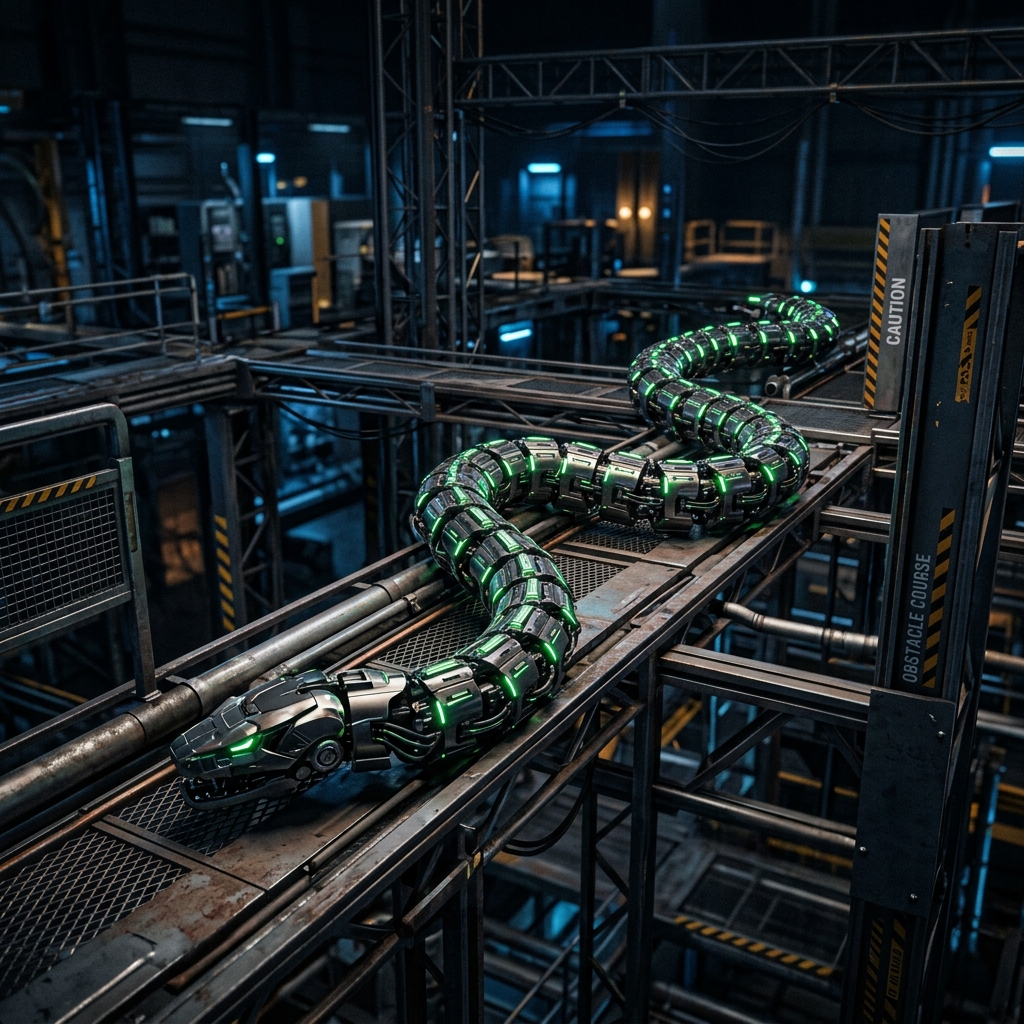
Redundancy Resolution and Locomotion Gaits of Hyper-Redundant Snake Robots: Jacobian Pseudoinverse and Obstacle-Aided Motion

Section 1: Introduction and Mathematical Modeling of Kinematic Redundancy

1.1 Biological Inspiration: Ophidian Locomotion and the Engineering Transition

The study of snake locomotion, or ophidian movement, represents one of the most compelling examples of functional morphology and biomechanics in the natural world. Biological snakes (suborder Serpentes) are characterized by a limbless, highly articulated skeletal structure containing between 130 and 500 vertebrae. Each vertebral joint is actuated by a complex, overlapping network of muscles that enables continuous, high-degree-of-freedom deformation. This unique morphology allows snakes to traverse diverse, highly irregular, and unstructured environments—such as dense vegetation, narrow rock crevices, unstable sand dunes, and tree branches—that present impassable obstacles to conventional wheeled, tracked, or legged organisms.

The biological spine of a snake is driven by a sophisticated muscular system consisting of epaxial (above the ribs) and hypaxial (below the ribs) muscle groups. These muscles, such as the semispinalis-spinalis and the longissimus dorsi, span across multiple vertebrae (sometimes up to 30 vertebral segments), creating a highly coordinated system of distributed force generation. This anatomical redundancy allows the snake to smoothly control its curvature profile, distributing pressure evenly along its body to prevent stress concentration at any single joint.

Biological snakes have evolved several distinct locomotion gaits, each optimized for specific substrate conditions and environmental constraints. The four primary gaits include:

• Lateral Undulation (Serpentine Locomotion): The most common snake gait, characterized by a continuous, wave-like bending of the body that propagates from head to tail. To generate forward thrust, the snake requires lateral contact points (e.g., rocks, twigs, or soil irregularities) against which the body can push. The physical secret behind lateral undulation lies in the anisotropic friction properties of the snake's ventral scales.

  At a microscopic level, scanning electron microscopy (SEM) reveals that these scales are covered by an array of tiny, backward-pointing spiny projections called micro-fibrils. These micro-fibrils typically have a length of $2$ to $5\ \mu\text{m}$, a width of approximately $0.2\ \mu\text{m}$, and a spatial density of around $10^6$ to $10^7$ per square millimeter. When the snake moves forward (longitudinal motion), these fibrils lie flat against the scale surface, resulting in a low sliding friction coefficient (typically $\mu_l \approx 0.1 \text{ to } 0.15$). However, when the body slides laterally or backward (transverse motion), the fibrils bend, stand up, and catch on the micro-roughness of the substrate. This interlocking mechanism creates a high transverse friction coefficient (typically $\mu_t \approx 0.3 \text{ to } 0.5$). The anisotropy ratio $\mu_t / \mu_l$ typically ranges between 2.0 and 5.0 on natural substrates. This difference allows the snake to slip forward along its own body curve while resisting lateral sliding, converting lateral muscular force into net forward propulsion.

  In robotic simulations and dynamic modeling, this anisotropic friction is mathematically represented to capture the interaction between each robot link and the environment. Under a viscous friction model, the friction force $F_{f, i}$ acting on the center of mass of the $i$-th link is formulated as:

  $$ F_{f, i} = -c_l \left( \dot{p}_i^T t_i \right) t_i - c_t \left( \dot{p}_i^T n_i \right) n_i $$

  where $\dot{p}_i \in \mathbb{R}^2$ is the velocity of the center of mass of link $i$, while $t_i = [\cos\phi_i, \sin\phi_i]^T$ and $n_i = [-\sin\phi_i, \cos\phi_i]^T$ are the unit tangent and unit normal vectors to the link's longitudinal axis, respectively. The positive constants $c_l$ and $c_t$ represent the longitudinal and transverse friction coefficients. By enforcing $c_t \gg c_l$, any lateral movement of the link is heavily damped and resisted by the ground, while longitudinal movement along the body curve is permitted with minimal resistance, thereby translating internal joint undulations into net forward translation.

• Concertina Locomotion: Typically employed in narrow tunnels, crevices, or when climbing vertical surfaces. When using this gait, the snake anchors the posterior part of its body by pressing it laterally against the walls of the channel (creating static contact), then extends the anterior portion forward. Once the anterior section is extended, it is anchored to the walls, and the posterior section is released and pulled forward. This bellows-like motion is energetically expensive but highly effective in confined spaces. The mechanics of concertina locomotion rely on generating a normal wall force $F_n$ large enough to ensure that the static friction limit $\mu_s F_n$ exceeds the gravitational and forward resistive forces acting on the extending body segments. Mathematically, if $M_{ant}$ is the mass of the anterior extended section, and $g$ is the gravitational acceleration, the normal anchoring force $F_n$ must satisfy:
  $$ \mu_s F_n \ge M_{ant} g + F_{res} $$
  where $F_{res}$ represents the resistance of the path ahead. This requires precise coordination between the loop-anchoring muscles and the extending spinal segments.
• Sidewinding: Optimized for low-friction or highly unstable substrates, such as loose sand. In sidewinding, the snake moves laterally across the ground by lifting sections of its body off the substrate, leaving a series of parallel, diagonal tracks. The body remains in static contact with the ground at only two moving contact zones, minimizing sliding friction and preventing the snake from sinking into loose sand. The physics of sidewinding involve the coordination of two orthogonal waves: a horizontal bending wave and a vertical lifting wave, phase-shifted by $\pi/2$ (or $90^\circ$). The segments in contact with the ground experience zero slipping, which prevents shear failure of the loose substrate and minimizes thermal energy transfer from hot desert sands.
• Rectilinear Locomotion: Primarily used by heavy-bodied snakes (such as large pythons and boas) for slow, straight-line movement. The snake uses its ribs and ventral skin scales to create linear waves of contraction and expansion that travel from head to tail, pulling the body forward incrementally. This gait relies on the elasticity of the ventral skin and the direct coordination of costocutaneous muscles, allowing the snake to move through narrow passages without lateral body sway.

The engineering transition from biological agents to hyper-redundant serial robots is motivated by the desire to replicate this level of mobility. Traditional robotic systems with a small number of degrees of freedom (DoF) struggle in unstructured environments due to their rigid kinematic constraints. In contrast, a snake-like robot consists of a large number of active links connected in series, providing a massive redundancy of joints. Shigeo Hirose's pioneering work in the 1970s with the construction of the Active Cord Mechanism (ACM-III) demonstrated that serpentine motion could be achieved by using a series of active joints equipped with passive wheels to enforce anisotropic friction constraints. Hirose formulated the serpenoid curve, a mathematical function describing the curvature profile of a planar snake during lateral undulation, showing that a sinusoidal distribution of joint angles generates smooth, natural serpentine gaits. Subsequent work by Gregory Chirikjian and Joel Burdick formalized the "backbone curve" framework, enabling the kinematic analysis of hyper-redundant systems by mapping a continuous virtual backbone curve to a discrete physical link structure.

1.2 Hirose's Serpenoid Curve and Bessel Function Representation

To capture the mathematical essence of lateral undulation, Shigeo Hirose proposed that the body curve of a snake moving on a flat plane can be modeled by a curve whose curvature changes sinusoidally with respect to the arc length. This curve is defined as the serpenoid curve. Let $s' \in [0, S]$ represent the arc length along the backbone curve of the snake, where $S$ is the total body length. The curvature $\kappa(s')$ at any point $s'$ is expressed as:

where $\kappa_0$ represents the maximum curvature and $a$ is the spatial frequency of the body wave. The angle $\theta_{tan}(s')$ of the tangent vector to the curve at arc length $s'$ relative to the global coordinate axis is obtained by integrating the curvature:

By adjusting the reference frame so that the initial angle term cancels, we can write the tangent angle profile in a simplified form:

where $\theta_0$ is the winding angle of the serpentine gait, representing the maximum angle that any body segment makes with the net direction of locomotion. The Cartesian coordinates $x(s')$ and $y(s')$ of the points along the snake's body are obtained by integrating the trigonometric functions of the tangent angle:

These integrals do not possess simple closed-form expressions in terms of elementary functions. To evaluate them analytically, we employ the Jacobi-Anger expansion, which decomposes trigonometric functions of sine waves into infinite series of Bessel functions of the first kind:

where $J_n(\theta_0)$ represents the Bessel function of the first kind of order $n$. Substituting these expansions into the coordinate integrals and performing term-by-term integration yields:

The term $J_0(\theta_0) s'$ in the $x(s')$ equation represents the linear progression of the snake along the primary axis of motion. Since $|J_0(\theta_0)| \le 1$ for all $\theta_0$, this shows that the forward progress is scaled by the zeroth-order Bessel function, indicating that a larger winding angle $\theta_0$ increases the lateral width of the gait but reduces the forward progress per unit of body length.

1.3 Kinematic Redundancy and Hyper-Redundancy: Mathematical Formulation

To analyze the kinematics of a robotic system, we define the mapping between the configuration space (joint space) and the task space. Let $\mathcal{Q} \subset \mathbb{R}^n$ represent the joint configuration space, where $n$ is the number of independent, active degrees of freedom. A configuration is represented by the joint coordinate vector:

Let $\mathcal{X} \subset \mathbb{R}^m$ represent the task space, which defines the coordinates of interest for the task (for example, the position and orientation of the end-effector or head of the robot). A task coordinate vector is represented by:

The forward kinematic mapping is a non-linear vector function $f: \mathcal{Q} \to \mathcal{X}$ that maps joint coordinates to task coordinates:

A robotic manipulator is classified based on the relationship between the joint space dimension $n$ and the task space dimension $m$:

• Kinematic Redundancy: Occurs when the number of joint degrees of freedom is strictly greater than the number of dimensions required to define the task ($n > m$). The difference $r = n - m$ is defined as the degree of redundancy.
• Hyper-Redundancy: Occurs when the degree of redundancy is extremely large ($n \gg m$, typically $n \ge 12$ for a 3-dimensional task space where $m = 6$).

The existence of kinematic redundancy has profound topological implications for the configuration space. For a given desired task space target $x_{e,d} \in \mathcal{X}$, the set of all joint configurations $\theta$ that achieve this target is the preimage of $x_{e,d}$ under the mapping $f$:

Under the assumption that $x_{e,d}$ is a regular value of the mapping $f$, the Jacobian matrix $J(\theta) = \frac{\partial f(\theta)}{\partial \theta}$ has full row rank $m$ for all configurations $\theta \in \mathcal{M}_{\text{self}}$. According to the Implicit Function Theorem, the preimage $\mathcal{M}_{\text{self}}$ is a differentiable submanifold of the configuration space $\mathcal{Q}$ of dimension $r = n - m$. This submanifold is known as the self-motion manifold or the fiber of the kinematic map.

1.4 Planar vs. Three-Dimensional Representations

When modeling snake robots, we must choose between planar (2D) and spatial (3D) kinematic representations. The choice represents a trade-off between mathematical simplicity and physical locomotory capability.

Planar Snake Robots: In a planar representation, all joint axes of rotation are assumed to be parallel to one another and perpendicular to the ground plane (typically the $z$-axis). Consequently, the motion of the entire robot is restricted to a 2D plane ($xy$-plane). The task space dimension is typically $m = 2$ (Cartesian position of the end-effector) or $m = 3$ (position and orientation in $SE(2)$).

The advantages of the planar model include:

1. Simplified Kinematics: Since the joint axes are parallel, the forward kinematics reduce to cumulative 2D rotations, eliminating the need for full $SO(3)$ rotation matrices.
2. Reduced Dynamic Complexity: The absence of gravitational torque variations out of the plane simplifies the dynamic equations of motion, making it easier to study wave propagation, scale-friction models, and propulsion forces.

However, planar robots are limited in their physical capabilities: they cannot lift sections of their body off the ground to navigate rugged terrain, climb pipes, or perform out-of-plane maneuvers like sidewinding.

Three-Dimensional Snake Robots: A spatial snake robot is typically constructed using a modular architecture with alternating orthogonal joints. For example, joint $1$ rotates about the $z$-axis (yaw), joint $2$ rotates about the $y$-axis (pitch), joint $3$ about the $z$-axis, and so on. This alternating configuration allows the robot to bend in both horizontal and vertical planes simultaneously. The task space is defined in $SE(3)$, with $m = 6$ (three translation dimensions and three orientation dimensions).

Spatial representations are necessary for analyzing complex locomotion gaits such as:

• Helical climbing: Wrapping the robot's body around a cylinder and propagating a spatial wave to climb vertically.
• Sidewinding: Coordinating horizontal and vertical waves with a phase shift (typically $90^\circ$) to lift segments of the body dynamically.
• Obstacle navigation: Climbing over barriers or entering complex 3D pipe structures.

The cost of this spatial capability is a highly non-linear forward kinematic map, a susceptibility to self-collision, and a complex Jacobian matrix with coupling between out-of-plane joint motions.

1.5 Continuous Backbone Curves vs. Discrete Kinematics

In the path planning of hyper-redundant serial robots, analyzing the individual links directly can lead to highly complex formulations due to the large number of joints. To resolve this complexity, Chirikjian and Burdick introduced the continuous backbone curve framework. Rather than planning the motion of each discrete link segment, the robot's shape is modeled using a continuous space curve, and the actual joint angles are extracted by fitting the physical links to this curve.

Let $r(s') \in \mathbb{R}^3$ represent a spatial curve parameterized by the arc length $s' \in [0, S]$, where $S$ is the total length of the snake's body. To completely define the spatial orientation of the snake robot's body along this curve, we attach a local frame $R(s') \in SO(3)$ to each point of the curve. The geometry of the curve is governed by the Frenet-Serret equations or by specifying three continuous deformation functions: extension $u(s')$, curvature functions $\kappa_1(s')$ and $\kappa_2(s')$, and torsion $\tau(s')$.

To constrain the shapes of the backbone curve to a lower-dimensional representation, the deformation functions are expanded using a set of modal shape functions:

where $\{\psi_j(s')\}$ is a set of predefined modes (such as Fourier modes, Legendre polynomials, or Chebyshev polynomials), $\{a_j\}$ is a vector of modal participation coefficients, and $M \ll n$ is the number of modes. By restricting the shape of the continuous backbone to a small number of modes $M$, we reduce the dimensionality of the path planning problem. Once the optimal modal coefficients $\{a_j\}$ are computed, the corresponding discrete joint angles $\theta_i$ of the physical robot are calculated by minimizing the geometric fitting error between the physical joints and the continuous curve:

where $p_i(\theta)$ is the position of joint $i$ derived from the forward kinematics, and $r(s'_i)$ is the corresponding target point on the continuous backbone curve.

The Sampling-Based Fitting Technique for Planar Kinematics

To understand how the continuous backbone curve is converted into joint angles without executing expensive numerical optimization, let us examine the case of a planar snake robot. Suppose the robot has $N$ rigid links of equal length $L = S/N$. The shape of a continuous planar backbone curve is completely defined by its tangent angle function $\theta_{tan}(s')$ with respect to the horizontal axis, where $s' \in [0, S]$.

We expand the tangent angle function using a modal decomposition over $M$ shape modes:

where $a_j$ are the modal participation factors and $\psi_j(s')$ are the orthonormal modal shape functions. For example, if we use a Fourier sine basis:

The Cartesian coordinates of the points along this continuous curve, $r(s') = [x(s'), y(s')]^T$, are obtained by integrating the tangent vector:

Chirikjian and Burdick demonstrated that for a planar, modular hyper-redundant robot, an excellent discrete approximation to the backbone curve can be obtained by directly sampling the continuous tangent angle function at the midpoint of each physical link segment. Specifically, the center of the $i$-th link corresponds to the arc length:

Under this sampling scheme, the absolute orientation $\phi_i$ of the $i$-th link relative to the global $x$-axis is set equal to the continuous tangent angle evaluated at $s'_i$:

Once the absolute link orientations $\{\phi_i\}$ are determined, the relative joint angles $\{\theta_i\}$ are calculated directly by taking the differences between adjacent link angles:

This formulation represents a significant breakthrough: it maps the continuous shape space parameters $a = [a_1, \dots, a_M]^T \in \mathbb{R}^M$ directly and algebraically to the joint coordinates $\theta = [\theta_1, \dots, \theta_N]^T \in \mathbb{R}^N$. Since $M \ll N$ (for example, controlling a 30-link robot using only $M = 4$ shape modes), the path planning and control calculations are restricted to a low-dimensional modal space, eliminating the computational complexity associated with high-dimensional joint spaces.

Spatial Aliasing and the Nyquist Constraint in Backbone Fitting

The sampling-based fitting method requires that the discrete link structure has sufficient spatial resolution to represent the shapes defined by the continuous backbone curve. Because sampling the continuous tangent angle $\theta_{tan}(s')$ is equivalent to uniform sampling in the spatial domain, we must consider the effects of spatial aliasing.

According to the Nyquist-Shannon sampling theorem applied to spatial coordinates, to reconstruct a continuous signal containing spatial frequency components up to $f_{\max}$ without aliasing, the sampling frequency $f_s$ must satisfy $f_s > 2 f_{\max}$. In the context of a discrete snake robot:

• The spatial sampling interval is the link length $L$, which corresponds to a spatial sampling frequency of $f_s = 1/L = N/S$ (samples per unit length).
• The spatial frequency of the $j$-th shape mode $\psi_j(s') = \sin\left( \frac{j \pi s'}{S} \right)$ is $f_j = \frac{j}{2S}$ (cycles per unit length).
• The highest spatial frequency component present in the continuous shape profile is $f_{\max} = f_M = \frac{M}{2S}$.

To prevent spatial aliasing—where high-frequency shape modes are folded back and incorrectly reconstructed as low-frequency joint movements—the sampling frequency must exceed the Nyquist rate:

Physically, this constraint dictates that the number of discrete robot links $N$ must be strictly greater than the number of active shape modes $M$. If $N \le M$, the robot lacks the necessary degrees of freedom to replicate the curvature changes of the continuous curve, leading to severe geometric fitting errors and physical distortion of the intended gait. In practice, a higher margin is preferred (such as $N \ge 3M$) to ensure that the discrete links fit the continuous curve smoothly and to minimize the spatial discretization error.

1.6 Kinematics of an N-Link Serial Snake Robot ($N \ge 12$)

Let us formulate the kinematics of a general $N$-link serial snake-like robot. Let $N$ be a large integer representing a hyper-redundant configuration, such as $N \ge 12$. The robot consists of $N$ rigid, homogeneous links connected in series by $N$ revolute joints.

Let us first consider a planar model to establish the analytical framework. Let $l_i$ represent the length of link $i$ (for $i = 1, 2, \dots, N$). The joints are indexed from $1$ to $N$, with joint $1$ connecting the base (or the tail) to the first link, and joint $N$ connecting link $N-1$ to the final link $N$. The configuration of the robot is described by the joint coordinate vector:

where $\theta_i$ represents the relative angle between link $i$ and link $i-1$. Let $\theta_1$ represent the absolute orientation of the first link relative to the global coordinate frame's positive $x$-axis.

Let $\phi_i$ represent the absolute orientation of link $i$ relative to the global $x$-axis. The absolute orientation of each link is the cumulative sum of the relative joint angles up to that link:

Let the origin of the base frame be $p_0 = [x_0, y_0]^T = [0, 0]^T$. The position of the joint $i$ (the connection point between link $i$ and link $i+1$) in the global frame, denoted by $p_i = [x_i, y_i]^T$, is derived recursively:

The end-effector (or head of the robot) is located at the tip of the $N$-th link. Its position $p_e = [x_e, y_e]^T$ and orientation $\phi_e$ are given by:

Thus, the forward kinematic mapping $f(\theta) = [x_e, y_e, \phi_e]^T$ maps the $N$-dimensional joint space to a 3-dimensional task space ($m = 3$):

For a spatial 3D snake robot, the recursive coordinate transformation uses homogeneous transformation matrices. Let $\{i\}$ be the coordinate frame attached to link $i$. The homogeneous transformation matrix $T_i^{i-1}(\theta_i)$ maps coordinates from frame $\{i\}$ to frame $\{i-1\}$:

where $R_i^{i-1}(\theta_i) \in SO(3)$ is the rotation matrix, and $p_{i/i-1}^{i-1} \in \mathbb{R}^3$ is the translation vector. The cumulative transformation from the end-effector frame $\{N\}$ to the base frame $\{0\}$ is:

where:

with $R_0^0 = I_{3\times3}$ and $R_{i-1}^0 = \prod_{k=1}^{i-1} R_k^{k-1}$.

1.7 The Curse of Dimensionality and the Velocity-Level Redundancy Resolution Paradigm

As the number of links $N$ increases to achieve high adaptability and flexibility, the configuration space $\mathcal{Q}$ grows in dimension. Path planning and trajectory generation for hyper-redundant robots become mathematically and computationally challenging due to the curse of dimensionality.

Consider the task of finding a collision-free path in a configuration space of dimension $N \ge 12$:

1. Grid-Based Planners: Classical grid-based search methods (e.g., Dijkstra's algorithm, A*) discretize each dimension of the configuration space. If each joint angle is discretized into $k$ intervals, the total number of grid states is $k^N$. For $N = 12$ and a coarse discretization of $k = 10$, the search space contains $10^{12}$ states. Searching this grid requires computational resources that scale exponentially, rendering real-time applications impossible.
2. Sampling-Based Planners: Algorithms such as Rapidly-exploring Random Trees (RRT) and Probabilistic Roadmaps (PRM) avoid discretization by sampling configurations randomly. While effective at finding paths in high-dimensional spaces, sampling-based methods are computationally expensive and do not guarantee smoothness. The resulting joint trajectories are often jerky, which can excite high-frequency dynamics in the robot's physical structure and cause actuator wear. Enforcing smooth velocities requires post-processing optimization, adding further computational overhead.
3. Global Trajectory Optimization: Methods that optimize the entire trajectory over a time horizon (e.g., using Pontryagin's Minimum Principle or direct collocation) must solve large-scale non-linear programming (NLP) problems. These methods are prone to local minima and are typically too slow for real-time control loops.

To achieve real-time control, researchers utilize the **velocity-level (differential) redundancy resolution** paradigm. By differentiating the forward kinematic map $x_e = f(\theta)$ with respect to time, we obtain:

where $\dot{x}_e \in \mathbb{R}^m$ is the task space velocity vector, $\dot{\theta} \in \mathbb{R}^n$ is the joint velocity vector, and $J(\theta) \in \mathbb{R}^{m \times n}$ is the Jacobian matrix.

At any given instant, the configuration $\theta$ is known, and $\dot{x}_e = J(\theta) \dot{\theta}$ represents a system of linear equations. Because $n > m$, this linear system is underdetermined, admitting infinitely many solutions for the joint velocities $\dot{\theta}$. Solving this system requires linear algebraic operations (such as computing the pseudoinverse of $J(\theta)$), which scale as $O(n^3)$ using standard matrix operations. For $N = 12$ or even $N = 100$, an $O(n^3)$ computation takes less than a millisecond on a modern processor, enabling real-time control loops operating at 1 kHz.

Furthermore, differential kinematics allows us to naturally incorporate secondary objectives by decomposing the joint velocities into a minimum-norm tracking term and a self-motion term. Using the null-space projection of the Jacobian, we can track the primary task exactly while simultaneously using the internal degrees of freedom to optimize potential functions (e.g., avoiding joint limits, avoiding obstacles, or maintaining high manipulability). This local, linear algebraic formulation bypasses the curse of dimensionality, transforming a global non-linear optimization problem into a sequence of local linear operations.

Section 2: Kinematic Formulations and the Jacobian Matrix

2.1 Denavit-Hartenberg (D-H) Parameterization of a Modular 3D Snake Robot

To establish a systematic kinematic model of a modular 3D snake robot, we employ the Denavit-Hartenberg (D-H) parameterization. The robot is modeled as a serial chain of rigid links connected by revolute joints. To achieve full 3D mobility, the robot features a modular structure with alternating orthogonal joint axes: pitch joints (which allow bending in the vertical plane) and yaw joints (which allow bending in the horizontal plane).

Let us define the coordinate frames according to the standard D-H convention. The $z_{i-1}$ axis is aligned with the axis of rotation of joint $i$. The $x_i$ axis is defined along the common normal from $z_{i-1}$ to $z_i$, pointing from joint $i$ to joint $i+1$. The origin $o_i$ is at the intersection of $z_i$ and $x_i$. The transformation between frame $\{i-1\}$ and frame $\{i\}$ is parameterized by four variables:

1. Joint angle $\theta_i$: The angle of rotation about $z_{i-1}$, measured from $x_{i-1}$ to $x_i$.
2. Link offset $d_i$: The distance along $z_{i-1}$ from the origin $o_{i-1}$ to the intersection of the $z_{i-1}$ and $x_i$ axes.
3. Link length $a_i$: The distance along $x_i$ from the intersection of the $z_{i-1}$ and $x_i$ axes to the origin $o_i$.
4. Link twist $\alpha_i$: The angle of rotation about $x_i$, measured from $z_{i-1}$ to $z_i$.

Consider a modular 3D snake robot consisting of $N$ modules. Each module has a physical length $L$. We assign a pitch joint (odd indices, $i = 2k-1$) and a yaw joint (even indices, $i = 2k$). The rotation axes of the pitch and yaw joints are perpendicular to each other.

To model this alternating orthogonal structure:

• The joint axes alternate orientations. For a pitch joint, the axis of rotation $z_{2k-2}$ is horizontal. For a yaw joint, the axis of rotation $z_{2k-1}$ is vertical.
• To transition the axis orientation, the twist angle $\alpha_i$ alternates between $\pi/2$ and $-\pi/2$.
• Since the joints are aligned along the longitudinal axis of each module with no lateral offset, the link offsets are $d_i = 0$ for all $i$.
• The link length $a_i = L$ represents the physical length of each module segment.

The D-H parameters for this modular 3D snake robot are summarized in Table 2:

Table 2: D-H Parameters for a Modular 3D Snake Robot with Pitch-Yaw Joints

Link ($i$)	Joint Type	Joint Angle ($\theta_i$)	Link Offset ($d_i$)	Link Length ($a_i$)	Link Twist ($\alpha_i$)
1	Pitch	$\theta_1$ (Variable)	0	$L$	$\pi/2$
2	Yaw	$\theta_2$ (Variable)	0	$L$	$-\pi/2$
3	Pitch	$\theta_3$ (Variable)	0	$L$	$\pi/2$
4	Yaw	$\theta_4$ (Variable)	0	$L$	$-\pi/2$
$\vdots$	$\vdots$	$\vdots$	$\vdots$	$\vdots$	$\vdots$
$2k-1$	Pitch	$\theta_{2k-1}$ (Variable)	0	$L$	$\pi/2$
$2k$	Yaw	$\theta_{2k}$ (Variable)	0	$L$	$-\pi/2$
$\vdots$	$\vdots$	$\vdots$	$\vdots$	$\vdots$	$\vdots$
$N$	Pitch/Yaw	$\theta_N$ (Variable)	0	$L$	$\alpha_N$

2.2 Derivation of Forward Kinematics via Homogeneous Transformation Matrices

The Homogeneous Transformation Matrix $T_i^{i-1}$ maps vectors from the coordinate frame $\{i\}$ to frame $\{i-1\}$. It is derived by multiplying the individual matrices for each D-H parameter transformation:

Substituting the basic transformation matrices:

Let us perform the matrix multiplication in steps:

Substituting the D-H parameters for our modular snake robot ($d_i = 0$, $a_i = L$):

• For Pitch Joints ($i = 2k-1$, where $\alpha_i = \pi/2$):
  $$ T_{2k-1}^{2k-2} = \begin{bmatrix} \cos\theta_{2k-1} & 0 & \sin\theta_{2k-1} & L \cos\theta_{2k-1} \\ \sin\theta_{2k-1} & 0 & -\cos\theta_{2k-1} & L \sin\theta_{2k-1} \\ 0 & 1 & 0 & 0 \\ 0 & 0 & 0 & 1 \end{bmatrix} $$
• For Yaw Joints ($i = 2k$, where $\alpha_i = -\pi/2$):
  $$ T_{2k}^{2k-1} = \begin{bmatrix} \cos\theta_{2k} & 0 & -\sin\theta_{2k} & L \cos\theta_{2k} \\ \sin\theta_{2k} & 0 & \cos\theta_{2k} & L \sin\theta_{2k} \\ 0 & -1 & 0 & 0 \\ 0 & 0 & 0 & 1 \end{bmatrix} $$

The cumulative transformation matrix from the end-effector frame $\{N\}$ to the base frame $\{0\}$ is:

The position of the end-effector in the base coordinate system is extracted from the upper-right $3 \times 1$ subvector of $T_N^0(\theta)$:

The orientation of the end-effector is represented by the rotation matrix $R_N^0(\theta) \in SO(3)$:

To express the task space coordinates in a vector format $x_e = f(\theta)$, we can choose Z-Y-X Euler angles (roll $\phi$, pitch $\theta_y$, yaw $\psi$) to represent the orientation:

where the Euler angles are extracted from the rotation matrix $R_N^0$:

Section 2: Kinematic Formulations and the Jacobian Matrix

2.3 The Jacobian Matrix: Analytical and Geometric Formulations

The relationship between joint velocities and task space velocities is governed by the Jacobian matrix. We must distinguish between the geometric Jacobian $J_g(\theta)$ and the analytical Jacobian $J(\theta)$.

The geometric Jacobian maps joint velocities to the physical linear velocity $v_e \in \mathbb{R}^3$ and angular velocity $\omega_e \in \mathbb{R}^3$ of the end-effector:

where $J_g(\theta) \in \mathbb{R}^{6 \times N}$. Since all joints of the snake robot are revolute, the $i$-th column of $J_g(\theta)$, denoted by $J_{g,i}$, is:

where:

Here, $z_{i-1}$ is the unit vector along the rotation axis of joint $i$, expressed in the base frame. It is the third column of the rotation matrix $R_{i-1}^0$:

and $p_{i-1}$ is the position vector of the origin of frame $\{i-1\}$ in the base frame, extracted from the first three elements of the fourth column of $T_{i-1}^0$.

Derivation of the Geometric Jacobian columns

Let us prove the column formulations using rigid body kinematics. The position of the end-effector in the base frame is:

where $p_{e/i-1}^{i-1}$ is the position of the end-effector relative to frame $\{i-1\}$, expressed in frame $\{i-1\}$ coordinates. Differentiating $p_e$ with respect to time, and considering only the motion of joint $i$ (with all other joints locked):

Since all preceding joints are locked, $\dot{p}_{i-1} = 0$ and $\dot{R}_{i-1}^0 = 0$. The relative position vector in frame $\{i-1\}$ changes due to the rotation of joint $i$ about the $z$-axis of frame $\{i-1\}$ with velocity $\dot{\theta}_i$. In frame $\{i-1\}$, this velocity is:

Multiplying by $R_{i-1}^0$ to transform this velocity to the base frame:

Using the property that rotation distributes over cross product, i.e., $R(a \times b) = (Ra) \times (Rb)$:

We identify that $R_{i-1}^0 [0, 0, 1]^T = z_{i-1}$ and $R_{i-1}^0 p_{e/i-1}^{i-1} = p_e - p_{i-1}$. Substituting these terms:

This proves that the contribution of joint $i$'s velocity to the linear velocity of the end-effector is $J_{P,i} = z_{i-1} \times (p_e - p_{i-1})$. Physically, this represents the cross product of the rotation axis vector $z_{i-1}$ with the lever arm vector $(p_e - p_{i-1})$ from the joint to the end-effector, yielding the tangential velocity direction and magnitude per unit joint speed.

For the angular velocity, the rotation of joint $i$ about $z_{i-1}$ adds an angular velocity component directly along the axis $z_{i-1}$:

Thus, $J_{O,i} = z_{i-1}$. Summing the contributions of all joints yields the complete geometric Jacobian $J_g(\theta)$.

Example: Analytical Jacobian of a Three-Link Planar Robot

To make this formulation concrete, let us derive the exact Jacobian matrix for a 3-link planar manipulator ($n = 3$) tracking a 2D position target ($m = 2$). The link lengths are $l_1, l_2, l_3$, and the joint angles are $\theta_1, \theta_2, \theta_3$. The absolute orientation angles of the links are:

The forward kinematic equations for the end-effector position $p_e = [x_e, y_e]^T$ are:

The analytical Jacobian $J(\theta) \in \mathbb{R}^{2 \times 3}$ is obtained by taking the partial derivatives of $x_e$ and $y_e$ with respect to $\theta_1, \theta_2, \theta_3$:

Computing the derivatives:

This gives the analytical Jacobian:

where $s_1 = \sin(\theta_1)$, $s_{12} = \sin(\theta_1 + \theta_2)$, $s_{123} = \sin(\theta_1+\theta_2+\theta_3)$, and similarly for the cosine terms. We can check that this matches the geometric Jacobian columns $J_{P,i} = z_{i-1} \times (p_e - p_{i-1})$ where the rotation axes are $z_0 = z_1 = z_2 = [0, 0, 1]^T$.

Analytical Jacobian Formulation

The analytical Jacobian $J(\theta)$ is defined by differentiating the end-effector pose vector $x_e = [p_e^T, \phi_e^T]^T$ with respect to time:

where $\dot{\phi}_e = [\dot{\phi}, \dot{\theta}_y, \dot{\psi}]^T$ is the vector of Euler angle rates. The relationship between $\dot{\phi}_e$ and the physical angular velocity $\omega_e$ is linear and depends on the current orientation $\phi_e$:

Let us derive $E(\phi_e)$ for Z-Y-X Euler angles (where rotation is defined as $R = R_z(\psi) R_y(\theta_y) R_x(\phi)$). The angular velocity vector $\omega_e$ is the sum of the angular velocity components associated with the rate of change of each angle:

where:

• $z_0 = [0, 0, 1]^T$ is the original base $z$-axis.
• $y' = [-\sin\psi, \cos\psi, 0]^T$ is the intermediate $y$-axis after the yaw rotation $\psi$.
• $x'' = [\cos\theta_y \cos\psi, \cos\theta_y \sin\psi, -\sin\theta_y]^T$ is the final $x$-axis after the yaw and pitch rotations.

Expressing this sum in matrix form:

Thus, the mapping matrix $E(\phi_e)$ is:

The inverse relationship is:

where:

The analytical Jacobian $J(\theta)$ is related to the geometric Jacobian $J_g(\theta)$ by:

2.4 Kinematic Singularities and Yoshikawa's Manipulability Measure

A kinematic singularity is a configuration $\theta$ at which the Jacobian matrix $J(\theta) \in \mathbb{R}^{m \times n}$ loses rank:

At a singular configuration, the robot loses one or more degrees of freedom in the task space. Mathematically, this means the mapping $\dot{\theta} \to \dot{x}_e$ is no longer surjective, and there exists a task space direction along which the end-effector cannot move.

For a hyper-redundant robot, singularities can be classified into:

1. Boundary Singularities: Occur when the robot is fully stretched out or folded back on itself. In these configurations, the end-effector is at the boundary of its physical workspace, and motion in the direction normal to the boundary is physically impossible.
2. Internal Singularities: Occur within the workspace when two or more joint axes align, restricting motion in certain directions. For a hyper-redundant robot, because $n \gg m$, the robot has many internal degrees of freedom. This allows the robot to perform self-motions to escape or avoid internal singularities while keeping the end-effector at its desired position.

To quantify a configuration's distance from a singularity, Tsuneo Yoshikawa introduced the manipulability index $w(\theta)$:

Let us analyze the mathematical properties and physical meaning of $w(\theta)$. Consider the set of all joint velocities in the unit sphere:

Assuming $J(\theta)$ has full row rank $m$, the minimum-norm joint velocity that achieves a task velocity $\dot{x}_e$ is:

Substituting this into the unit sphere inequality:

This inequality defines a hyper-ellipsoid in the task space $\mathbb{R}^m$, known as the manipulability ellipsoid. The eigenvalues and eigenvectors of the symmetric matrix $J J^T \in \mathbb{R}^{m \times m}$ define the principal axes and orientations of this ellipsoid.

Let the singular value decomposition of $J(\theta)$ be:

where $U \in \mathbb{R}^{m \times m}$ and $V \in \mathbb{R}^{n \times n}$ are orthogonal matrices, and $\Sigma \in \mathbb{R}^{m \times n}$ contains the singular values $\sigma_1 \ge \sigma_2 \ge \dots \ge \sigma_m \ge 0$. The matrix $J J^T$ is:

The determinant is:

Therefore, the manipulability index $w(\theta)$ is:

The volume of the manipulability ellipsoid is proportional to the product of its semi-axes, which are the singular values $\sigma_i$. Hence, the manipulability index $w(\theta)$ is directly proportional to the volume of the ellipsoid.

• When $w(\theta)$ is large, the robot can generate high task-space velocities in all directions with relatively small joint velocities.
• When $w(\theta) = 0$, at least one singular value is zero, indicating a loss of rank. The ellipsoid collapses along the corresponding direction, and the robot is in a singular configuration.

For a hyper-redundant snake robot, keeping the configuraton far from singularities is essential. The high-dimensional self-motion manifold allows the robot to perform shape adjustments (self-motions) to maximize $w(\theta)$ while keeping the end-effector stationary.

2.5 Alternative Manipulability Measures: Condition Number and Minimum Singular Value

While Yoshikawa's manipulability index $w(\theta)$ is a widely used scalar measure for singularity proximity, it has certain limitations in control design. Because $w(\theta)$ is the product of all singular values, it can remain relatively large even if one of the singular values is very close to zero, provided that the other singular values are exceptionally large. This can lead to situations where the control system fails to recognize that the robot is approaching a singularity along a specific direction.

To address this, two alternative manipulability measures are commonly used:

1. Minimum Singular Value ($\sigma_{\min}(J)$): The value of $\sigma_{\min}(J)$ represents the distance of the Jacobian matrix from the space of rank-deficient matrices in terms of the spectral norm. It defines the worst-case velocity transmission capability of the robot. If $\sigma_{\min}(J) \to 0$, the robot is approaching a singularity, regardless of how large the other singular values are. Mathematically, it measures the radius of the smallest axis of the manipulability ellipsoid.
2. Condition Number ($\kappa(J)$): The condition number of the Jacobian matrix is defined as the ratio of the maximum singular value to the minimum singular value:
   $$ \kappa(J) = \|J\|_2 \|J^+\|_2 = \frac{\sigma_{\max}(J)}{\sigma_{\min}(J)} $$
   The condition number ranges from $1$ to $\infty$. A configuration where $\kappa(J) = 1$ is called isotropic. In an isotropic configuration, the manipulability ellipsoid is a perfect sphere, meaning the robot can move its end-effector with equal ease in all directions. If $\kappa(J) \to \infty$, the robot is in a singular configuration. In control systems, minimizing the condition number (or maximizing its reciprocal $\kappa^{-1}(J) \in [0, 1]$) is a robust way to ensure uniform velocity capability and avoid numerical instability in the pseudoinverse calculation.

   A high condition number indicates that command inputs along the weakest axis will be mapped to extremely large joint velocities, while inputs along the strongest axis require virtually no joint motion. This asymmetry can lead to severe joint tracking errors in discrete-time controllers and degrades the numerical accuracy of standard ODE integrators (such as Euler or Runge-Kutta) used in real-time simulation.

From a force transmission perspective, we can define the force manipulability ellipsoid:

where $F \in \mathbb{R}^m$ is the force/torque vector applied at the end-effector, mapped from the joint torques $\tau = J^T F$. The eigenvalues of $J J^T$ are the squared singular values $\sigma_i^2$. This reveals a fundamental duality between velocity and force transmission:

Section 3: Redundancy Resolution via the Jacobian Pseudoinverse

3.1 Velocity-Level Redundancy Resolution as a Constrained Optimization Problem

For a kinematically redundant robot ($n > m$), the differential kinematic relationship $J(\theta) \dot{\theta} = \dot{x}_e$ represents an underdetermined system of linear equations. To select a unique joint velocity vector $\dot{\theta}$ from the infinite set of valid solutions, we formulate the selection as a constrained optimization problem.

Let us define a quadratic cost function that minimizes the weighted norm of the joint velocities:

where $W \in \mathbb{R}^{n \times n}$ is a symmetric, positive-definite weighting matrix. The weighting matrix $W$ allows us to penalize the movement of specific joints. For instance, we can assign larger weights to joints near the base of the robot to restrict their motion, or to joints with smaller actuator limits.

The optimization problem is formulated as:

We solve this problem using the method of Lagrange multipliers. Let $\lambda \in \mathbb{R}^m$ be the vector of Lagrange multipliers. The Lagrangian function is:

To find the optimal joint velocity vector, we compute the partial derivatives of $L(\dot{\theta}, \lambda)$ with respect to $\dot{\theta}$ and $\lambda$ and set them to zero:

Since $W$ is positive-definite, it is invertible. From Equation 1, we solve for $\dot{\theta}$:

Substituting Equation 3 into the constraint (Equation 2):

Since $J$ has full row rank $m$ and $W^{-1}$ is positive-definite, the matrix $(J W^{-1} J^T) \in \mathbb{R}^{m \times m}$ is symmetric, positive-definite, and invertible. Solving for $\lambda$:

Substituting this back into Equation 3 yields the optimal joint velocity solution:

This defines the weighted pseudoinverse $J_W^+ \in \mathbb{R}^{n \times m}$:

yielding:

3.2 The Moore-Penrose Pseudoinverse and Null-Space Projection

In the unweighted case where $W = I$ (the identity matrix), all joints are penalized equally. The cost function reduces to the squared Euclidean norm of the joint velocities:

Under this condition, the weighted pseudoinverse $J_W^+$ simplifies to the standard Moore-Penrose pseudoinverse $J^+$:

The joint velocity solution is:

Proof of Minimality of the Moore-Penrose Solution

Let $\dot{\theta}$ be any joint velocity vector satisfying $J \dot{\theta} = \dot{x}_e$. We decompose $\dot{\theta}$ into two components:

where:

Let us verify the properties of these two components:

1. First, verify that $\dot{\theta}_p$ satisfies the tracking constraint:
   $$ J \dot{\theta}_p = J J^+ \dot{x}_e = J J^T (J J^T)^{-1} \dot{x}_e = I_m \dot{x}_e = \dot{x}_e $$
2. Second, verify that $\dot{\theta}_n$ lies in the null space of $J$ (i.e., $J \dot{\theta}_n = 0$):
   $$ J \dot{\theta}_n = J (I - J^+ J) \dot{\theta} = (J - J J^+ J) \dot{\theta} $$
   Substituting $J^+ = J^T (J J^T)^{-1}$:
   $$ J J^+ J = J \left( J^T (J J^T)^{-1} \right) J = (J J^T)(J J^T)^{-1} J = I_m J = J $$
   Therefore:
   $$ J \dot{\theta}_n = (J - J) \dot{\theta} = 0 $$
   This confirms that $\dot{\theta}_n \in \mathcal{N}(J)$.
3. Third, show that $\dot{\theta}_p$ and $\dot{\theta}_n$ are orthogonal:
   $$ \dot{\theta}_p^T \dot{\theta}_n = \left( J^+ \dot{x}_e \right)^T \left( (I - J^+ J) \dot{\theta} \right) = \dot{x}_e^T (J^+)^T (I - J^+ J) \dot{\theta} $$
   Expanding the transpose of the pseudoinverse:
   $$ (J^+)^T = \left( J^T (J J^T)^{-1} \right)^T = (J J^T)^{-T} J = (J J^T)^{-1} J $$
   Substituting this back:
   $$ (J^+)^T (I - J^+ J) = (J J^T)^{-1} J (I - J^T (J J^T)^{-1} J) $$
   $$ = (J J^T)^{-1} J - (J J^T)^{-1} J J^T (J J^T)^{-1} J $$
   $$ = (J J^T)^{-1} J - (J J^T)^{-1} I_m J = 0 $$
   Thus, $\dot{\theta}_p^T \dot{\theta}_n = 0$.

Now, we calculate the squared Euclidean norm of $\dot{\theta}$:

Since the cross-product term is zero:

Because $\|\dot{\theta}_n\|^2 \ge 0$, it follows that:

with equality holding if and only if $\dot{\theta}_n = 0$. This completes the proof that $\dot{\theta}_p = J^+ \dot{x}_e$ is the unique solution that minimizes the Euclidean norm of the joint velocities.

Null-Space Projection and the General Redundancy Resolution Solution

The orthogonality between the tracking solution and the null-space components allows us to formulate the general solution to the redundancy resolution problem:

where $q_0 \in \mathbb{R}^n$ is an arbitrary joint velocity vector representing a secondary objective, and $P_{\text{null}} = (I - J^+ J) \in \mathbb{R}^{n \times n}$ is the null-space projection operator.

Let us verify that this general solution satisfies the primary tracking constraint for any choice of $q_0$:

The projection matrix $P_{\text{null}}$ filters out any components of $q_0$ that would cause the end-effector to move, leaving only the "self-motion" components.

The operator $P_{\text{null}} = I - J^+ J$ possesses two key mathematical properties:

1. Symmetry:
   $$ P_{\text{null}}^T = (I - J^+ J)^T = I - (J^+ J)^T = I - J^T (J^+)^T $$
   Substituting $(J^+)^T = (J J^T)^{-1} J$:
   $$ P_{\text{null}}^T = I - J^T (J J^T)^{-1} J = I - J^+ J = P_{\text{null}} $$
2. Idempotency:
   $$ P_{\text{null}}^2 = (I - J^+ J)(I - J^+ J) = I - 2 J^+ J + J^+ J J^+ J $$
   Recall that $J^+ J J^+ = J^+$. Multiplying by $J$ on the right:
   $$ J^+ J J^+ J = J^+ J $$
   Substituting this back:
   $$ P_{\text{null}}^2 = I - 2 J^+ J + J^+ J = I - J^+ J = P_{\text{null}} $$

An operator that is both symmetric and idempotent is an orthogonal projection operator. Thus, $P_{\text{null}}$ projects vectors orthogonally onto the null space of the Jacobian.

3.3 Singularity-Robust Pseudoinverse (Damped Least-Squares)

While the Moore-Penrose pseudoinverse provides the minimum-norm joint velocity solution, it suffers from severe numerical instability in the vicinity of kinematic singularities. When the robot configuration $\theta$ approaches a singularity, at least one of the singular values $\sigma_i$ of the Jacobian approaches zero. Since the pseudoinverse contains terms scaling as $1/\sigma_i$, the joint velocities calculated via $\dot{\theta} = J^+ \dot{x}_e$ grow boundlessly. Physically, this leads to actuator saturation, structural vibration, and potential mechanical failure.

To address this issue, we can relax the exact tracking constraint using a multi-objective optimization problem. We define the cost function:

where $k > 0$ is a damping factor. This formulation represents a trade-off: the first term minimizes the tracking error, while the second term (the damping term) penalizes large joint velocities. This approach is mathematically equivalent to Tikhonov regularization or the Levenberg-Marquardt algorithm.

Let us derive the solution by expanding the quadratic terms:

Differentiating $E(\dot{\theta})$ with respect to the joint velocity vector $\dot{\theta}$ and setting it to zero:

Solving for $\dot{\theta}$ yields:

Although this formula is mathematically correct, it requires inverting an $n \times n$ matrix, which is computationally expensive for hyper-redundant robots with a large number of links $n \gg m$. To improve computational efficiency, we use the matrix identity:

Proof of the Damped Pseudoinverse Identity

Let us prove this identity by showing that multiplying both sides by the corresponding inverse terms yields the same result. Let:

We multiply $X$ on the left by $(J^T J + k^2 I_n)$ and $Y$ on the right by $(J J^T + k^2 I_m)$:

Now, performing the same operations for $Y$:

Since both expressions result in $J^T J J^T + k^2 J^T$, the identity is proven.

Using this identity, the singularity-robust pseudoinverse solution can be written as:

where $J^* = J^T (J J^T + k^2 I_m)^{-1}$ is the singularity-robust pseudoinverse. This formulation only requires inverting an $m \times m$ matrix (typically $6 \times 6$), which is computationally efficient.

Physically, the damped least-squares solution behaves as if virtual linear springs are attached between the end-effector and the target trajectory, while virtual dampers are attached to all joints in the joint space. The damping factor $k$ regulates the stiffness of these virtual joint dampers. Choosing $k$ requires balancing tracking accuracy and joint velocity limits: if $k$ is too small, joint velocities still exceed physical limits near singularities; if $k$ is too large, the tracking error becomes unacceptable even when the robot is far from singularities.

To minimize tracking error in non-singular regions while ensuring stability near singularities, we can dynamically adjust the damping factor $k^2$ based on the manipulability index $w(\theta)$:

where $w_0$ is a user-defined threshold and $k_0$ is the maximum damping factor applied at the singularity.

3.4 Formulation of Secondary Objectives

To utilize the null-space projection term, we design the secondary vector $q_0$ using potential functions. Let $H(\theta)$ be a scalar potential function representing a secondary objective we wish to minimize. We set:

where $k_{\text{sec}} > 0$ is a scalar gain, and $\nabla H(\theta) \in \mathbb{R}^n$ is the gradient of $H$ with respect to the joint angles:

This choice of $q_0$ performs gradient descent on $H(\theta)$ within the null space, driving the joint configuration towards local minima of $H(\theta)$ without affecting the end-effector trajectory. Conversely, to maximize a potential function $w(\theta)$ (such as manipulability), we perform gradient ascent:

We now formulate three critical secondary objectives for hyper-redundant snake robots:

1. Joint Limit Avoidance

Physical snake robots have mechanical limits on their joint angles. Let the upper and lower limits for joint $i$ be $\theta_{i,\max}$ and $\theta_{i,\min}$, respectively. To prevent joints from reaching these limits, we define a potential function $H(\theta)$ that penalizes proximity to the boundaries.

A standard approach uses a normalized squared distance potential:

where $\bar{\theta}_i$ is the midpoint of the joint range:

The gradient of this potential function with respect to joint $\theta_i$ is:

While simple to compute, this potential function remains finite at the limits. To create a strict barrier, we can use a reciprocal barrier potential function:

This potential function has the following properties:

• At the midpoint $\theta_i = \bar{\theta}_i$, the potential is $H_i(\bar{\theta}_i) = 1$.
• As joint $\theta_i$ approaches either limit ($\theta_{i,\max}$ or $\theta_{i,\min}$), the denominator approaches zero, causing the potential to go to infinity ($H_i \to \infty$).

Let us derive the gradient of this barrier potential with respect to $\theta_i$:

Using the chain and product rules:

Computing the derivative of the term in brackets:

Substituting this back:

Alternatively, we can use a logarithmic barrier function, which is commonly used in interior-point optimization methods:

The gradient of this logarithmic barrier function with respect to $\theta_i$ is:

When $\theta_i = \bar{\theta}_i$ (at the joint midpoint), this gradient becomes zero:

This property is ideal: when the joints are centered, the gradient is zero, generating no null-space velocity and leaving the primary task tracking completely unaffected. As a joint approaches its limits, the corresponding gradient term grows rapidly, pushing the joint away from the limit.

Using either barrier gradient in the null-space projection term:

effectively prevents the joint coordinates from reaching their physical limits.

2. Singularity Avoidance

To keep the robot far from singular configurations, we maximize Yoshikawa's manipulability index $w(\theta) = \sqrt{\det(J(\theta) J(\theta)^T)}$ by performing gradient ascent:

To calculate $\nabla w(\theta)$, we need the partial derivatives $\frac{\partial w(\theta)}{\partial \theta_i}$. Let $M(\theta) = J(\theta) J(\theta)^T \in \mathbb{R}^{m \times m}$. Thus, $w(\theta) = \sqrt{\det(M(\theta))}$. Using the chain rule:

According to Jacobi's formula, the derivative of the determinant of a matrix $M$ with respect to a scalar parameter $\theta_i$ is:

Substituting this back:

Next, we expand the derivative of the product $J J^T$:

Using the properties of the trace operator ($\text{tr}(A+B) = \text{tr}(A) + \text{tr}(B)$ and $\text{tr}(A^T) = \text{tr}(A)$):

Since $(J J^T)^{-1}$ is symmetric:

Using the cyclic permutation property of the trace ($\text{tr}(ABC) = \text{tr}(CAB)$):

Thus, the two terms are identical:

Substituting this result back into the derivative of $w(\theta)$ yields:

This provides a closed-form analytical expression for the gradient of the manipulability index. It depends on the partial derivative of the Jacobian matrix, $\frac{\partial J}{\partial \theta_i}$.

3.5 Advanced Null-Space Formulations: Analytical Derivatives of the Geometric Jacobian

To evaluate the analytical gradient of the manipulability index without relying on finite differences, we must derive the analytical derivative of the geometric Jacobian matrix, $\frac{\partial J_g}{\partial \theta_j}$.

Let $J_{g, i}$ represent the $i$-th column of the geometric Jacobian $J_g \in \mathbb{R}^{6 \times n}$:

We want to compute the partial derivative $\frac{\partial J_{g, i}}{\partial \theta_j}$ for all $i, j \in \{1, 2, \dots, n\}$. We analyze this by considering the topological structure of the serial kinematic chain:

1. Case 1: $j > i$ (Perturbation is downstream of the joint axis):

   If joint $j$ is downstream of joint $i$, a change in the joint angle $\theta_j$ does not affect the orientation of the joint axis $z_{i-1}$ or the position of the joint origin $p_{i-1}$. However, it does affect the position of the end-effector $p_e$. Thus:

   $$ \frac{\partial z_{i-1}}{\partial \theta_j} = 0 \quad \text{and} \quad \frac{\partial p_{i-1}}{\partial \theta_j} = 0 $$
   Applying these derivatives to the column vector:
   $$ \frac{\partial J_{g, i}}{\partial \theta_j} = \begin{bmatrix} z_{i-1} \times \frac{\partial p_e}{\partial \theta_j} \\ 0_{3\times1} \end{bmatrix} $$
   Recall that the derivative of the end-effector position with respect to joint $\theta_j$ is the linear velocity column of the Jacobian:
   $$ \frac{\partial p_e}{\partial \theta_j} = z_{j-1} \times (p_e - p_{j-1}) $$
   Substituting this back:
   $$ \frac{\partial J_{g, i}}{\partial \theta_j} = \begin{bmatrix} z_{i-1} \times \left( z_{j-1} \times (p_e - p_{j-1}) \right) \\ 0_{3\times1} \end{bmatrix} \quad \text{for } j > i $$
2. Case 2: $j \le i$ (Perturbation is upstream of the joint axis):

   If joint $j$ is upstream of (or equal to) joint $i$, a rotation of joint $j$ rotates the entire downstream kinematic chain, including the axis $z_{i-1}$, the position $p_{i-1}$, and the end-effector position $p_e$, as a rigid body about the axis $z_{j-1}$.

   For any vector $v$ that is rigidly attached to the chain downstream of joint $j$, its derivative with respect to $\theta_j$ is:
   $$ \frac{\partial v}{\partial \theta_j} = z_{j-1} \times v $$
   Applying this rule to the unit vector $z_{i-1}$ and the relative position vectors:
   $$ \frac{\partial z_{i-1}}{\partial \theta_j} = z_{j-1} \times z_{i-1} $$
   $$ \frac{\partial p_{i-1}}{\partial \theta_j} = z_{j-1} \times (p_{i-1} - p_{j-1}) $$
   $$ \frac{\partial p_e}{\partial \theta_j} = z_{j-1} \times (p_e - p_{j-1}) $$
   We derive the derivative of the linear velocity term $J_{P, i} = z_{i-1} \times (p_e - p_{i-1})$ using the product rule:
   $$ \frac{\partial J_{P, i}}{\partial \theta_j} = \frac{\partial z_{i-1}}{\partial \theta_j} \times (p_e - p_{i-1}) + z_{i-1} \times \left( \frac{\partial p_e}{\partial \theta_j} - \frac{\partial p_{i-1}}{\partial \theta_j} \right) $$
   Substituting the derivatives:
   $$ \frac{\partial J_{P, i}}{\partial \theta_j} = (z_{j-1} \times z_{i-1}) \times (p_e - p_{i-1}) + z_{i-1} \times \left[ z_{j-1} \times (p_e - p_{j-1}) - z_{j-1} \times (p_{i-1} - p_{j-1}) \right] $$
   Using the linearity of the cross product:
   $$ \frac{\partial J_{P, i}}{\partial \theta_j} = (z_{j-1} \times z_{i-1}) \times (p_e - p_{i-1}) + z_{i-1} \times \left[ z_{j-1} \times (p_e - p_{i-1}) \right] $$
   Thus, the column derivative is:
   $$ \frac{\partial J_{g, i}}{\partial \theta_j} = \begin{bmatrix} (z_{j-1} \times z_{i-1}) \times (p_e - p_{i-1}) + z_{i-1} \times \left[ z_{j-1} \times (p_e - p_{i-1}) \right] \\ z_{j-1} \times z_{i-1} \end{bmatrix} \quad \text{for } j \le i $$

These expressions provide the exact analytical derivatives of the geometric Jacobian. This avoids the numerical errors associated with finite difference approximations, ensuring stable control updates when maximizing manipulability in the null space.

3. Obstacle Avoidance

To prevent the snake robot's body from colliding with workspace obstacles, we implement artificial potential fields. Let $x_{\text{obs}} \in \mathbb{R}^3$ be the coordinates of an obstacle.

Because a snake robot has a distributed body, we must protect the entire structure from collisions rather than just the end-effector. We select a set of $K$ control points distributed along the robot's body. Let $x_k(\theta) \in \mathbb{R}^3$ represent the position of the $k$-th control point (for example, at the center of mass of link $k$).

For each control point $x_k$ and obstacle $x_{\text{obs}}$, the distance is:

We define a repulsive potential $U_{\text{obs}, k}(\theta)$ that increases as the control point approaches the obstacle:

where $\eta > 0$ is a scaling gain and $\rho_0 > 0$ is the barrier's influence distance. The total obstacle potential is:

To minimize this potential, we perform gradient descent in the null space:

We calculate the gradient $\nabla U_{\text{obs}, k}(\theta)$ using the chain rule:

where:

• $J_k(\theta) = \frac{\partial x_k(\theta)}{\partial \theta} \in \mathbb{R}^{3 \times n}$ is the position Jacobian of control point $x_k$. Note that since $x_k$ is located on link $k$, its position depends only on the first $k$ joint variables. Thus, columns $k+1$ to $N$ of $J_k(\theta)$ are zero vectors.
• $\nabla_{x_k} U_{\text{obs}, k}$ is the gradient of the potential with respect to the Cartesian coordinates of $x_k$:
  $$ \nabla_{x_k} U_{\text{obs}, k} = \frac{\partial}{\partial x_k} \left[ \frac{1}{2} \eta \left( \frac{1}{\|x_k - x_{\text{obs}}\|} - \frac{1}{\rho_0} \right)^2 \right] $$
  Letting $d = \|x_k - x_{\text{obs}}\|$:
  $$ \nabla_{x_k} U_{\text{obs}, k} = \eta \left( \frac{1}{d} - \frac{1}{\rho_0} \right) \frac{\partial}{\partial x_k} \left( \frac{1}{\|x_k - x_{\text{obs}}\|} \right) $$
  Since:
  $$ \frac{\partial}{\partial x_k} \left( \frac{1}{\|x_k - x_{\text{obs}}\|} \right) = -\frac{x_k - x_{\text{obs}}}{d^3} $$
  We have:
  $$ \nabla_{x_k} U_{\text{obs}, k} = -\eta \left( \frac{1}{d} - \frac{1}{\rho_0} \right) \frac{x_k - x_{\text{obs}}}{d^3} $$

Substituting this back into the joint-space gradient:

The total gradient is:

Thus, the obstacle avoidance null-space vector is:

In practical implementations, to find the closest point $x_k$ on a cylindrical link segment $[p_{i-1}, p_i]$ to a spherical obstacle $x_{\text{obs}}$, we project the obstacle position orthogonally onto the line segment representing the link axis. Let $u = \frac{p_i - p_{i-1}}{\|p_i - p_{i-1}\|}$ be the unit direction vector of the link. The projection parameter $t$ is:

We clamp $t$ to the range $[0, 1]$ to ensure the point lies within the physical link boundaries:

The closest point on the link axis to the obstacle is:

By evaluating the Jacobian $J_k(\theta)$ of this dynamically selected closest point, the obstacle avoidance vector $q_0$ pushes the link away from the obstacle.

4. Hierarchical Redundancy Resolution (Multi-Task Framework)

When a hyper-redundant robot must perform multiple secondary tasks simultaneously (e.g., tracking a trajectory while avoiding obstacles and avoiding joint limits), simply summing the null-space vectors $q_0 = q_{0, \text{obs}} + q_{0, \text{limit}} + q_{0, \text{sing}}$ can cause conflicts. For instance, the joint limit avoidance task might push a link into an obstacle, or vice versa.

To resolve this, we utilize a hierarchical redundancy resolution framework based on task priorities. Let the tasks be ordered by priority, where Task 1 is the primary end-effector tracking task, Task 2 is obstacle avoidance (highest secondary priority), and Task 3 is joint limit avoidance.

The joint velocity vector is computed recursively:

where $J_k$ is the Jacobian of the $k$-th task, $\dot{x}_{k, d}$ is the desired velocity for the $k$-th task, and $P_{k-1}$ is the orthogonal projector onto the intersection of the null spaces of all higher-priority tasks from $1$ to $k-1$:

with $P_0 = I$. This recursive formulation ensures that lower-priority tasks are executed entirely within the null spaces of all higher-priority tasks. As a result, the robot will prioritize avoiding obstacles over avoiding joint limits, and both tasks are guaranteed not to interfere with the primary tracking of the end-effector.