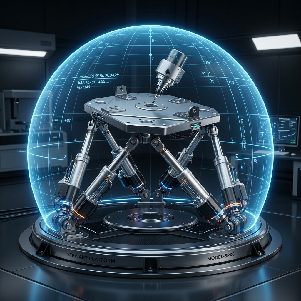
Singularity Analysis and Workspace Optimization of Parallel Manipulators (Stewart Platforms)

Section 1: Introduction to Parallel Manipulators

1.1 Paradigm Shift: Serial vs. Parallel Kinematic Chains

In the historical development of robotics and automated mechanisms, serial manipulators have served as the dominant paradigm. An open-loop serial kinematic chain is characterized by a sequence of rigid links connected by active joints—typically revolute or prismatic—stretching from a single fixed base to an end-effector. Representative designs such as the PUMA 560, SCARA configurations, and anthropomorphic robotic arms exhibit kinematic configurations where each joint must support the cumulative physical mass of all subsequent links, actuators, and transmission systems, in addition to the external payload. Consequently, these serial structures behave mechanically as cantilever beams. As the distance from the base increases, the bending moments and torsional stresses escalate quadratically, causing significant elastic deflections and structural vibrations under high-speed or heavy-load operations.

To counteract these structural deflections and maintain satisfactory precision at the end-effector, engineers must design serial robot links with substantial cross-sectional areas and high mass. This massive construction leads to an extremely unfavorable payload-to-weight ratio, which typically hovers between $1:10$ and $1:20$ (i.e., a robot weighing 200 kg is required to manipulate a payload of only 10 to 20 kg). Furthermore, the positioning errors of serial manipulators are cumulative. Any angular deviation or compliance in the joints near the base is amplified by the downstream link lengths, leading to substantial absolute errors at the end-effector.

Parallel manipulators represent a fundamental departure from this open-loop cantilever paradigm. A parallel manipulator is defined as a closed-loop kinematic chain in which a single moving platform is connected to a fixed base through two or more independent, closed kinematic branches (legs or struts). Because the load is shared across multiple parallel paths, the internal forces within the struts are primarily restricted to axial tension and compression, eliminating the dominant bending moments that plague serial arms. This load sharing allows parallel mechanisms to be constructed with lightweight structural members while maintaining exceptional stiffness-to-weight ratios. The payload-to-weight ratio of a parallel manipulator frequently exceeds $1:1$, and in heavy-duty industrial configurations, it can surpass $5:1$, representing an order-of-magnitude performance improvement.

Furthermore, parallel mechanisms exhibit excellent dynamic characteristics. The actuators can be mounted on or near the fixed base, drastically reducing the moving mass of the linkages. This minimized rotational and translational inertia enables extremely high accelerations and rapid, high-frequency dynamic responses. In terms of precision, parallel manipulators act as error-averaging mechanisms rather than error-accumulating ones. A small positioning error in one actuator does not propagate linearly; instead, the closed-loop constraints distribute the error across all joints, resulting in superior positioning repeatability and sub-micron resolution.

However, the advantages of parallel manipulators are balanced by severe trade-offs. The most notable limitation is their restricted workspace. While a serial arm can sweep out a vast spherical or toroidal volume relative to its physical footprint, a parallel manipulator is confined to a small, complex, and highly non-convex workspace. This restriction is dictated by physical leg interference (where the struts collide with one another), joint angle limitations at the base and platform connections, and the presence of complex internal singular configurations. Additionally, the closed-loop topology makes the forward kinematics—computing the position and orientation of the platform given the leg lengths—computationally difficult and mathematically multi-valued, requiring robust numerical search methods for real-time control.

Table 1: Structural and Performance Comparison of Serial and Parallel Manipulators

Performance Indicator	Serial Manipulator (Open-Loop)	Parallel Manipulator (Closed-Loop)
Topology	Open kinematic chain	Closed kinematic chain
Structural Loading	Cantilever bending, torsion, shear	Axial tension and compression
Payload-to-Weight Ratio	Low (typically 1:10 to 1:20)	High (often 1:1 to 5:1 or higher)
Structural Stiffness	Low to moderate (limited by bending stiffness)	Extremely high (axial stiffness of struts)
Dynamic Performance	Limited by high moving mass of actuators	Excellent (actuators near base, low moving mass)
Error Propagation	Cumulative (additive along the chain)	Averaging (errors distributed across loops)
Workspace Volume	Large, spherical/toroidal, simple boundary	Small, highly restricted, complex boundary
Kinematics Complexity	Simple forward, complex inverse kinematics	Complex forward, simple inverse kinematics

1.2 Historical Context and Evolution: The Gough-Stewart Platform

The genesis of parallel robotics lies in the mid-20th century. The earliest mathematical and physical conceptualization of a six-degree-of-freedom (6-DOF) parallel mechanism was developed by V.E. Gough, an engineer at the Dunlop Rubber Company in Birmingham, United Kingdom. In 1947, Gough sought to design a universal tyre testing machine capable of subjecting tyres to realistic, multi-axis forces and moments—including vertical loads, lateral forces, longitudinal forces, slip angles, and self-aligning torques. To apply these combined loads, Gough developed a mechanical platform supported by six adjustable-length struts, which was fully fabricated and operational by the early 1950s. This tyre tester represented the first practical implementation of a six-axis parallel mechanism, establishing the basic geometric layout of the modern hexapod.

Independently, D. Stewart published a seminal paper in 1965 titled "A Platform with Six Degrees of Freedom" in the Proceedings of the Institution of Mechanical Engineers. Stewart was searching for an effective mechanism to serve as a flight simulator motion base, recognizing that the rapid acceleration, heavy payload capacity, and high stiffness of parallel structures were ideally suited for replicating the inertial sensations of aircraft flight. Although Stewart’s original publication proposed a three-legged platform where each leg consisted of a coordinate mechanical arrangement (with two actuators per leg), he also proposed and discussed the six-legged configuration. Because of the parallel contribution of both engineers, this octahedral six-axis parallel manipulator is now universally referred to as the Gough-Stewart Platform.

Over the subsequent decades, the Gough-Stewart platform transitioned from flight simulation into diverse industrial and scientific applications. In the 1990s, the machine tool industry attempted to revolutionize machining with Parallel Kinematic Machines (PKMs), such as the Giddings & Lewis Variax and the Ingersoll Hexapod. Although these machines faced challenges—primarily due to the high variation in structural stiffness and accuracy across their workspace—they generated significant research in kinematic calibration, singular configuration avoidance, and workspace optimization. Today, Gough-Stewart platforms are deployed in high-precision environments, such as the positioning of sub-reflectors in astronomical radio telescopes (e.g., the ALMA observatory in Chile), surgical robotics (e.g., bone-mounted platforms for spinal surgery), semiconductor wafer positioning, and seismic test tables.

1.3 Mobility and Degrees of Freedom Analysis

To design and control a parallel manipulator, we must first establish its mobility, which represents the number of independent coordinates required to uniquely specify the mechanical configuration. In spatial mechanism theory, the mobility $M$ of a system is determined using the Chebychev-Kutzbach-Grübler (CKG) formula. For a general mechanism operating in a $d$-dimensional space, the mobility is given by:

where:
$\bullet$ $d$ is the dimensionality of the operational space ($d = 3$ for planar systems, $d = 6$ for general spatial systems),
$\bullet$ $n$ is the total number of links in the mechanism, including the fixed ground/base link,
$\bullet$ $g$ is the total number of joints,
$\bullet$ $f_i$ is the number of degrees of freedom permitted by the $i$-th joint.

Let us conduct a step-by-step mobility analysis of the standard 6-UPS Gough-Stewart platform using this spatial framework ($d = 6$). The architecture consists of a fixed base plate, a moving platform, and six identical, adjustable-length legs. Each leg is structured as a serial kinematic branch containing a universal joint, a prismatic joint, and a spherical joint.

First, we calculate the total number of links, $n$. The system comprises:
1. One fixed base (ground link): $1$,
2. One moving platform (end-effector): $1$,
3. Six legs, each containing two distinct rigid links: a lower leg cylinder and an upper sliding rod. This contributes $6 \times 2 = 12$ links.
Thus, the total link count is $n = 1 + 1 + 12 = 14$ links.

Second, we count the number of joints, $g$. Each of the six legs contains:
1. A Universal (U) joint connecting the lower leg to the base,
2. A Prismatic (P) joint connecting the lower leg to the upper rod,
3. A Spherical (S) joint connecting the upper rod to the moving platform.
This results in $g = 6 \text{ (universal)} + 6 \text{ (prismatic)} + 6 \text{ (spherical)} = 18$ joints.

Third, we evaluate the individual degrees of freedom $f_i$ for each joint type:
$\bullet$ A Universal joint is a 2-DOF joint, permitting two orthogonal rotations ($f_U = 2$),
$\bullet$ A Prismatic joint is a 1-DOF joint, allowing linear translation along the leg axis ($f_P = 1$),
$\bullet$ A Spherical joint is a 3-DOF joint, permitting rotation about three orthogonal axes ($f_S = 3$).

The sum of all joint degrees of freedom is computed as follows:

Substituting these values ($d = 6$, $n = 14$, $g = 18$, and $\sum f_i = 36$) into the CKG formula yields:

This mathematical result confirms that the standard 6-UPS Gough-Stewart platform has exactly 6 independent degrees of freedom, allowing arbitrary control of its position $(x, y, z)$ and orientation (defined by Roll-Pitch-Yaw angles).

To highlight the significance of the joint selection, let us analyze an alternative design: the 6-SPS platform. In this configuration, the universal joints at the base are replaced with spherical joints. The joint DOF count becomes:
$\bullet$ 12 spherical joints ($f_S = 3$),
$\bullet$ 6 prismatic joints ($f_P = 1$).
This changes the sum of the joint degrees of freedom:

Applying the CKG formula with $n = 14$, $g = 18$, and $\sum f_i = 42$:

The mobility of 12 indicates that the 6-SPS mechanism has 6 additional degrees of freedom beyond the 6 operational DOFs of the moving platform. These extra DOFs represent passive or idle motions. Specifically, each of the six struts can rotate freely about its own longitudinal axis (the line passing through the centers of its base and platform spherical joints). Although these passive rotations do not affect the translational or rotational state of the moving platform, they introduce practical engineering challenges. Leg-mounted components, such as linear encoders, load cells, or hydraulic supply hoses, are subjected to continuous twisting, which can lead to fatigue failure and electrical interference. To eliminate these passive motions, designers typically choose the 6-UPS topology or implement keyed prismatic joints that prevent rotation of the upper rod relative to the cylinder.

1.4 High-Performance Applications

The physical characteristics of parallel manipulators—high stiffness, massive payload capacity, and high dynamic response—make them indispensable in applications where serial robots are structurally inadequate.

Flight and Vehicle Motion Simulators: Replicating the dynamics of flight or high-speed driving requires a motion base that can support a heavy cabin (housing pilots, instrumentation, and visual displays) while executing high-frequency accelerations. To simulate gravity forces, turbulence, and sudden maneuvers, the motion base must possess high structural bandwidth. The Gough-Stewart platform is the industry standard for Category D flight simulators, providing the stiffness and dynamic response needed to reproduce 6-DOF inertial sensations.

Precision Optomechanical and Astronomical Alignment: In modern telescopes and optical systems, mirror segments must be aligned with sub-micron accuracy and maintained in position despite gravitational deformations and wind loading. Hexapods are used to adjust the secondary reflectors of large telescopes, where their high load capacity, high stiffness, and lack of backlash ensure stable, nanometer-level resolution.

Parallel Kinematic Machining: Traditional CNC milling machines rely on heavy orthogonal slides that stack axes serially, resulting in large moving masses. PKMs leverage the high stiffness of the Gough-Stewart platform to execute high-speed, 5-axis milling. The parallel struts carry primary axial loads, minimizing deflection under cutting forces and improving surface finish.

Medical and Surgical Robotics: In orthopedic and neurological surgeries, positioning accuracy is critical. Small, bone-mounted parallel robots provide a rigid, stable platform for surgical drills and guides. Their closed-loop structure prevents deflection when subjected to force, ensuring the tools follow the planned surgical trajectories.

Section 2: Forward and Inverse Kinematics

2.1 Coordinate Frame Setup and Kinematic Definitions

To establish a mathematical model of the Gough-Stewart platform, we define two coordinate frames:
1. The **base frame** $\{B\}$ is a fixed reference frame with origin $O_B$ located at a convenient reference point on the base plate. The axes of $\{B\}$ are denoted by $X_B, Y_B, Z_B$.
2. The **platform frame** $\{P\}$ is a moving coordinate frame attached to the moving platform, with origin $O_P$ typically situated at the platform's geometric center. The axes of $\{P\}$ are denoted by $X_P, Y_P, Z_P$.

The position of the moving platform relative to the base frame is defined by the translation vector $\mathbf{p} \in \mathbb{R}^3$, representing the coordinates of the origin $O_P$ in the base frame:

The orientation of the moving platform relative to the base frame is defined by the rotation matrix $R_P^B \in SO(3)$. This rotation matrix can be parameterized using Roll-Pitch-Yaw angles $(\phi, \theta, \psi)$, which represent sequential rotations about the axes of the base frame. We adopt the standard $Z\text{-}Y\text{-}X$ Euler angle convention (Yaw-Pitch-Roll):
1. First, rotate by Yaw angle $\psi$ about the $Z_B$ axis:

2. Second, rotate by Pitch angle $\theta$ about the intermediate $Y'$ axis:

3. Third, rotate by Roll angle $\phi$ about the intermediate $X''$ axis:

By composing these individual rotation matrices, we obtain the complete rotation matrix $R_P^B$:

Multiplying these matrices step-by-step:

Performing the final matrix multiplication yields:

Let the position of the base anchor point for the $i$-th leg in the base frame $\{B\}$ be represented by:

Similarly, let the position of the platform anchor point for the $i$-th leg, expressed relative to the platform frame $\{P\}$, be represented by:

Using the rotation matrix $R_P^B$ and translation vector $\mathbf{p}$, we transform the platform anchor points from the moving platform frame $\{P\}$ into the fixed base frame $\{B\}$:

2.2 Rigorous Derivation of Inverse Kinematics

The inverse kinematics problem for a parallel manipulator is defined as follows: given the desired position $\mathbf{p}$ and orientation $R_P^B$ of the moving platform, calculate the required active joint variables (the leg lengths $l_1, \dots, l_6$).

For each leg $i$, the leg vector $\mathbf{l}_i \in \mathbb{R}^3$, which points from the base anchor $\mathbf{b}_i$ to the corresponding platform anchor $\mathbf{p}_i$, is defined as:

The physical length $l_i$ of the $i$-th leg is the Euclidean norm of this vector:

To understand the algebraic behavior of the inverse kinematics, we expand this vector equation into its scalar components. Let us denote the elements of the rotation matrix $R_P^B$ as $R_{jk}$ ($j, k = 1, 2, 3$). The components of the transformed platform anchor point $\mathbf{p}_i = [x_{pi}, y_{pi}, z_{pi}]^T$ in the base frame are:

The components of the leg vector $\mathbf{l}_i = [l_{ix}, l_{iy}, l_{iz}]^T$ are:

By squaring the components and summing them, we obtain the squared leg length $l_i^2$:

Substituting the full parameterization of the rotation matrix $R_P^B$, we write the expanded algebraic expression for the squared length of the $i$-th leg:

Taking the square root of both sides gives the analytical solution for $l_i$. Since the leg lengths must be positive real numbers, the negative root is discarded. Unlike serial manipulators, which often require solving complex transcendental equations with multiple branch selections, the inverse kinematics of a parallel manipulator is decoupled: the length of each leg $l_i$ is computed independently. This simplicity makes the inverse kinematics computationally efficient for real-time control.

2.3 Forward Kinematics Challenges

The forward kinematics problem for the Gough-Stewart platform is stated as follows: given the six measured leg lengths $l_1, \dots, l_6$, find the position $\mathbf{p} = [x, y, z]^T$ and rotation matrix $R_P^B$ of the moving platform.

Geometrically, this problem is equivalent to finding the positions of the vertices of a rigid body (the platform) when each vertex is constrained to lie on a sphere of radius $l_i$ centered at the corresponding base anchor point $\mathbf{b}_i$. This leads to a system of six coupled, non-linear algebraic equations in six unknowns.

In contrast to serial manipulators, where forward kinematics is straightforward and inverse kinematics is challenging, parallel manipulators exhibit the opposite behavior. Analytical closed-form solutions for the general Gough-Stewart platform are difficult to obtain. In 1993, Raghavan and others demonstrated that the forward kinematics of the general parallel manipulator can be reduced to a 40th-degree univariate polynomial. This means that for a single set of leg lengths $l_i$, there can be up to 40 distinct real solutions, representing 40 different physical assembly modes.

These assembly modes represent different configurations in which the platform can be assembled with the same leg lengths. Many of these solutions are complex conjugate pairs or physically impossible configurations (e.g., configurations requiring the platform to pass through the base or self-intersect). However, multiple real, valid solutions can exist within the physical workspace. In real-time control applications, finding the unique physical pose corresponding to the current state of the robot is essential. Analytical methods based on elimination theory or Gröbner bases are computationally expensive and difficult to implement in real-time control loops, which requires the use of iterative numerical search algorithms.

2.4 Numerical Methods for Forward Kinematics: Newton-Raphson Method

To solve the forward kinematics problem in real time, we formulate it as a multi-dimensional root-finding problem and apply the Newton-Raphson method. Let the platform pose vector be defined by $\mathbf{x} = [x, y, z, \phi, \theta, \psi]^T \in \mathbb{R}^6$. Given the measured leg lengths $l_{i,\text{meas}}$ ($i = 1, \dots, 6$), we define a vector of residual functions $\mathbf{f}(\mathbf{x}) = [f_1(\mathbf{x}), \dots, f_6(\mathbf{x})]^T \in \mathbb{R}^6$:

where $\mathbf{l}_i(\mathbf{x}) = \mathbf{p} + R_P^B(\phi, \theta, \psi)\mathbf{p}_i^P - \mathbf{b}_i$. The Newton-Raphson method finds the root of this system by updating the pose estimate iteratively:

where $J_{\text{num}}(\mathbf{x}_k) \in \mathbb{R}^{6 \times 6}$ is the Jacobian matrix of the residual vector $\mathbf{f}$ evaluated at the current estimate $\mathbf{x}_k$:

To construct this Jacobian matrix, we calculate the partial derivatives of $f_i$ with respect to the elements of $\mathbf{x}$. For the translational variables $\mathbf{p} = [x, y, z]^T$:

This gives the first three columns of the Jacobian for row $i$:

For the rotational variables $\boldsymbol{\eta} = [\phi, \theta, \psi]^T$:

To calculate these derivatives, we derive the partial derivatives of the rotation matrix $R_P^B$ with respect to the Euler angles $\phi, \theta, \psi$. First, for the Roll angle $\phi$:

where:

Computing the matrix product:

Second, for the Pitch angle $\theta$:

where:

Computing the matrix product:

Third, for the Yaw angle $\psi$:

where:

Computing the matrix product:

This gives the complete formulation for the residual Jacobian matrix $J_{\text{num}}(\mathbf{x}_k)$. The algorithm for the Newton-Raphson search is detailed below:

Algorithm 1: Newton-Raphson Iteration for Stewart Platform Forward Kinematics
=============================================================================
Inputs:
  - Measured leg lengths: l_meas = [l_1, l_2, l_3, l_4, l_5, l_6]^T
  - Base anchor coordinates: b_i (for i = 1 to 6)
  - Platform anchor coordinates: p_i^P (for i = 1 to 6)
  - Initial pose estimate: x_0 = [x, y, z, phi, theta, psi]^T
  - Convergence tolerances: epsilon_1 (pose change), epsilon_2 (residual norm)
  - Maximum iterations: k_max

Initialization:
  Set k = 0
  x_k = x_0

Loop:
  1. Compute the rotation matrix R_P^B(phi_k, theta_k, psi_k)
  2. Compute the partial derivatives: dR/dphi, dR/dtheta, dR/dpsi
  
  3. Initialize the residual vector f = zeros(6, 1)
  4. Initialize the residual Jacobian J_num = zeros(6, 6)
  
  5. For each leg i = 1 to 6:
      a. Compute leg vector in base frame: 
         l_i = p_k + R_P^B * p_i^P - b_i
      b. Compute residual:
         f[i] = dot(l_i, l_i) - l_meas[i]^2
      c. Construct row i of J_num:
         J_num[i, 0] = 2 * l_i[0]  (d/dx)
         J_num[i, 1] = 2 * l_i[1]  (d/dy)
         J_num[i, 2] = 2 * l_i[2]  (d/dz)
         J_num[i, 3] = 2 * dot(l_i, (dR/dphi * p_i^P))
         J_num[i, 4] = 2 * dot(l_i, (dR/dtheta * p_i^P))
         J_num[i, 5] = 2 * dot(l_i, (dR/dpsi * p_i^P))

  6. Check convergence:
      If norm(f) < epsilon_2:
          Terminate and return x_k (Success)

  7. Solve the linear system for the update step delta_x:
      J_num * delta_x = -f
      (Implement via LU decomposition or QR factorization to avoid matrix inversion)

  8. Update the pose estimate:
      x_k1 = x_k + delta_x

  9. Check step size convergence:
      If norm(delta_x) < epsilon_1:
          Terminate and return x_k1 (Success)

  10. Update loop index:
      x_k = x_k1
      k = k + 1
      If k > k_max:
          Terminate and return failure (Divergence or Singularity)
=============================================================================

The Newton-Raphson method offers quadratic convergence near a root. In continuous control applications, the initial guess $\mathbf{x}_0$ is set to the estimated pose from the previous control cycle. Since the physical platform moves continuously, the pose change between cycles is small, allowing the algorithm to converge in 2 to 4 iterations.

However, if the initial guess is far from the true pose, the algorithm can diverge or converge to an incorrect assembly mode. Additionally, if the platform passes near a singular configuration, the Jacobian matrix $J_{\text{num}}$ becomes ill-conditioned, leading to numerical instability and search failure.

Section 3: Jacobian Formulation and Velocity Mapping

3.1 Velocity Kinematics and Definition of Twist

Velocity kinematics describes the mapping between the joint velocities of a manipulator and the velocity of its end-effector. For a six-degree-of-freedom parallel manipulator, the velocity of the moving platform is defined by the **twist vector** $\mathbf{t} \in \mathbb{R}^6$:

where:
$\bullet$ $\mathbf{v}_p = \dot{\mathbf{p}} = [\dot{x}, \dot{y}, \dot{z}]^T$ is the linear velocity of the moving platform origin $O_P$, expressed in the base frame $\{B\}$,
$\bullet$ $\boldsymbol{\omega}_p = [\omega_x, \omega_y, \omega_z]^T$ is the angular velocity vector of the moving platform, expressed in the base frame $\{B\}$.

The relationship between the time derivative of the rotation matrix $\dot{R}_P^B$ and the angular velocity vector $\boldsymbol{\omega}_p$ is given by:

where $[\boldsymbol{\omega}_p]_\times$ is the skew-symmetric matrix representation of the angular velocity vector $\boldsymbol{\omega}_p$:

To derive this relationship, we start with the orthogonality property of the rotation matrix:

Differentiating both sides of this equation with respect to time:

Rearranging terms:

This shows that the matrix $\Omega = \dot{R}_P^B (R_P^B)^T$ is equal to the negative of its transpose, which is the definition of a skew-symmetric matrix. Representing this matrix as $[\boldsymbol{\omega}_p]_\times$:

3.2 Velocity of the Platform Joint Anchors

The position of the $i$-th platform joint anchor in the base frame is defined as:

where $\mathbf{r}_i = R_P^B \mathbf{p}_i^P$ is the position vector of the platform joint relative to the origin of the platform frame, expressed in the base frame. Differentiating $\mathbf{p}_i$ with respect to time:

Since the coordinates of the platform joint in the moving frame ($\mathbf{p}_i^P$) are constant:

Substituting the relationship $\dot{R}_P^B = [\boldsymbol{\omega}_p]_\times R_P^B$:

Thus, the velocity of the $i$-th platform joint anchor in the base frame is:

3.3 Mapping Platform Twist to Leg Velocities

Next, we relate the velocity of the platform joints to the rate of change of the leg lengths (the active joint velocities). The leg vector is:

The square of the leg length is defined as:

Differentiating both sides of this equation with respect to time:

Defining the unit vector along the leg axis as $\hat{\mathbf{s}}_i = \frac{\mathbf{l}_i}{l_i}$:

Since the base anchors $\mathbf{b}_i$ are stationary in the base frame:

Substituting this and the expression for $\dot{\mathbf{p}}_i$ into the leg velocity equation:

Using the vector triple product property $\mathbf{a}^T (\mathbf{b} \times \mathbf{c}) = (\mathbf{c} \times \mathbf{a})^T \mathbf{b}$:

This gives the relationship for the rate of change of length for a single leg:

Writing this in matrix form:

3.4 Separation into Inverse and Forward Jacobians

By stacking the velocity equations for all six legs, we express the system of equations as:

In parallel robotics, the general relationship between joint rates $\dot{\mathbf{q}}$ and the platform twist $\mathbf{t}$ is written as:

where:
$\bullet$ $J_A$ is the **inverse Jacobian matrix**, which maps the joint rates to the constraint velocities,
$\bullet$ $J_B$ is the **forward Jacobian matrix**, which maps the platform twist to the constraint velocities.

For the standard 6-UPS Gough-Stewart platform, the active joint vector is $\mathbf{q} = \mathbf{l} = [l_1, \dots, l_6]^T$. Because the joint velocities are decoupled, $J_A$ is the identity matrix:

The forward Jacobian matrix $J_B \in \mathbb{R}^{6 \times 6}$ is:

The standard Jacobian matrix $J$, which directly relates the platform twist to the leg velocities ($\dot{\mathbf{l}} = J \mathbf{t}$), is given by:

To show the physical meaning of this separation, we analyze a configuration where $J_A$ is not the identity matrix. Consider a **rotary Stewart platform**, where the six legs are of fixed length $l_i$, and the platform is actuated by six rotary motors located at the base. Each motor drives an actuator arm of length $a_i$. The leg is connected to the tip of this arm via a universal joint.

Let the angle of the $i$-th actuator arm be denoted by $\theta_i$, and the position of the arm tip be $\mathbf{a}_i(\theta_i)$. The fixed-length leg constraint is:

where $\mathbf{l}_i = \mathbf{p}_i - \mathbf{a}_i(\theta_i) = \mathbf{p} + R_P^B \mathbf{p}_i^P - \mathbf{a}_i(\theta_i)$. Differentiating this constraint with respect to time:

The velocity of the actuator arm tip is:

where $\mathbf{d}_i$ is the velocity vector of the arm tip per unit joint rate. Substituting this and the platform joint velocity $\dot{\mathbf{p}}_i = \mathbf{v}_p + \boldsymbol{\omega}_p \times \mathbf{r}_i$:

Rearranging terms:

Dividing by the scalar leg length $l_i$ to introduce the unit direction vector $\hat{\mathbf{s}}_i = \frac{\mathbf{l}_i}{l_i}$:

Stacking these equations for all six legs gives the relationship:

where:

and $J_B$ remains identical to the forward Jacobian of the linear platform. This demonstration shows how the physical architecture determines the structure of $J_A$. In a rotary platform, $J_A$ is diagonal but depends on the robot's pose. If any diagonal element of $J_A$ becomes zero (which occurs when the leg vector is perpendicular to the velocity vector of the actuator arm tip), $J_A$ becomes singular. This condition represents a **Type I singularity**, where the platform loses a degree of freedom.

3.5 Duality of Force and Velocity (Statics Mapping)

The Jacobian matrix also defines the relationship between the joint forces and the forces and moments acting on the platform. Let the active forces applied along the six legs be denoted by the vector $\boldsymbol{\tau} = [f_1, f_2, \dots, f_6]^T \in \mathbb{R}^6$, where $f_i$ is the axial force in the $i$-th leg. Let the external load acting on the platform be defined by the wrench vector $\mathbf{w}_{\text{ext}} = [\mathbf{f}_{\text{ext}}^T, \mathbf{m}_{\text{ext}}^T]^T \in \mathbb{R}^6$, where $\mathbf{f}_{\text{ext}}$ is the net force and $\mathbf{m}_{\text{ext}}$ is the net moment acting about the origin $O_P$.

Under quasi-static conditions, we analyze the system using the **Principle of Virtual Work**. The virtual work $\delta W$ done by the external wrench and joint forces during a virtual displacement must sum to zero:

where $\delta \mathbf{x}_E = [\delta \mathbf{p}^T, \delta \boldsymbol{\theta}^T]^T$ is the virtual displacement of the platform and $\delta \mathbf{l}$ is the vector of virtual joint displacements. Substituting the velocity kinematics relationship $\delta \mathbf{l} = J \delta \mathbf{x}_E$:

Since this relationship must hold for any arbitrary virtual displacement $\delta \mathbf{x}_E$, the term inside the parentheses must be zero:

This equation shows the duality in the kinematics of the manipulator:
$\bullet$ The Jacobian matrix $J$ maps the platform velocities to the joint velocities: $\dot{\mathbf{l}} = J \mathbf{t}$.
$\bullet$ The transpose of the Jacobian matrix $J^T$ maps the active joint forces to the static wrench supported by the platform: $\mathbf{w}_{\text{ext}} = J^T \boldsymbol{\tau}$.

This static relationship is used to evaluate the load-carrying capacity of the manipulator and to design force-control algorithms. If the Jacobian matrix $J$ becomes singular, the platform can support external loads without generating forces in the active joints, or small external loads can produce large forces in the struts. This relationship is critical for identifying singular configurations, which are analyzed in subsequent sections.

Singularity Analysis and Workspace Optimization of Parallel Manipulators (Stewart Platforms)

Section 4: Numerical Worked Example

4.1 Geometric Parameters and Coordinate Reference Frames

To establish a concrete, physically realizable engineering application that highlights the kinematics and force-transmission relationships derived in the first part of this monograph, we present a comprehensive, step-by-step numerical worked example for a six-degree-of-freedom (6-DOF) spatial $6\text{-}\text{UPS}$ Gough-Stewart parallel manipulator. In industrial practice, parallel robots rarely utilize a fully symmetric circular arrangement of joint attachments where joint angles are spaced evenly at $60^\circ$ intervals. A fully symmetric circular distribution of joint connections leads to severe mathematical and physical limitations. In such configurations, the lines of action of the legs intersect in concentric alignments or form parallel planes under nominal configurations, creating permanent architectural singularities throughout the workspace. To prevent these configurations, engineers group the joints into three distinct pairs on both the base and the platform. This arrangement creates a stable, triangulated truss structure.

For this numerical case study, we define a medium-scale robotic motion platform, representing a flight simulator motion base or an active optical mirror support platform. The base radius $R_B$ represents the radial distance from the coordinate origin $O_B$ of the base frame $\{B\}$ to the center of each universal joint mounting point. The platform radius $R_P$ represents the radial distance from the local coordinate origin $O_P$ of the moving platform frame $\{P\}$ to the center of each spherical joint connection. The physical sizing parameters are:

The angular positions of the joint attachments on the base plate and moving platform are parameterized by half-angles that define the spacing between adjacent joints within a pair. Let $\theta_B$ define the base joint pair half-angle and $\theta_P$ define the platform joint pair half-angle. We select:

The angular coordinates $\theta_{B,i}$ for the base joint connections ($B_1$ to $B_6$) in the fixed coordinate frame $\{B\}$ are distributed symmetrically in pairs around the primary axes at $0^\circ, 120^\circ,$ and $240^\circ$:

To ensure a stable, triangulated truss structure, the platform joint angular coordinates $\theta_{P,i}$ ($P_1$ to $P_6$) in the local platform frame $\{P\}$ are also distributed in pairs but rotated by $60^\circ$ relative to the base configuration to create a stable, triangulated structure:

From these geometric parameters, the coordinates of the base anchor points $\mathbf{b}_i = [b_{x,i}, b_{y,i}, b_{z,i}]^T$ in the fixed frame $\{B\}$ and the platform anchor points in the local frame $\mathbf{p}_i = [p_{x,i}, p_{y,i}, p_{z,i}]^T$ in the platform frame $\{P\}$ are computed using planar transformations:

Evaluating these trigonometric expressions for all joint connections yields the spatial coordinates presented in Table 4.1.

Table 4.1: Coordinates of Base and Platform Joint Anchor Points (in meters)

Joint Index ($i$)	Base Anchor Position $\mathbf{b}_i$ in $\{B\}$	Platform Anchor Position $\mathbf{p}_i$ in $\{P\}$
1	$[0.482963, -0.129410, 0.000000]^T$	$[0.271892, 0.126785, 0.000000]^T$
2	$[0.482963, 0.129410, 0.000000]^T$	$[-0.026147, 0.298858, 0.000000]^T$
3	$[-0.129410, 0.482963, 0.000000]^T$	$[-0.245746, 0.172073, 0.000000]^T$
4	$[-0.353553, 0.353553, 0.000000]^T$	$[-0.245746, -0.172073, 0.000000]^T$
5	$[-0.353553, -0.353553, 0.000000]^T$	$[-0.026147, -0.298858, 0.000000]^T$
6	$[-0.129410, -0.482963, 0.000000]^T$	$[0.271892, -0.126785, 0.000000]^T$

4.2 Platform Pose Specification and Rotation Matrix Derivation

We define a target pose of the platform frame $\{P\}$ relative to the base frame $\{B\}$ through a translation vector $\mathbf{t}$ and a set of Roll-Pitch-Yaw angles. The selected pose represents a combination of translation, pitching, rolling, and yawing to simulate a typical operational state:

The orientation is expressed using the $Z\text{-}Y\text{-}X$ Euler angle sequence (yaw $\psi$, pitch $\theta$, roll $\phi$). This selection of Tait-Bryan angles is preferred in engineering kinematics because it aligns with standard aerospace and vehicular conventions, preventing mathematical ambiguities in nominal operational ranges.

The rotation matrix $R = R_z(\psi) R_y(\theta) R_x(\phi)$ is constructed by multiplying the individual rotation matrices:

Evaluating the trigonometric components:

This yields the numerical rotation matrix:

This matrix maps any vector from the local moving platform coordinates to the base reference coordinates. The orthogonality of the rotation matrix is verified by checking that $R R^T = I_{3 \times 3}$, confirming that the rotation preserves the rigid-body constraints of the moving platform.

4.3 Leg Vector and Actuator Length Resolution

For each actuator, the kinematics vector loop is written as:

Here, $\mathbf{q}_i$ represents the position of the platform joint in the base frame, $\mathbf{l}_i$ represents the leg vector pointing from the base anchor to the platform anchor, $l_i$ is the scalar leg length, and $\mathbf{s}_i$ is the unit direction vector along the leg axis. Geometrically, the leg vector represents the physical axis of the prismatic cylinder. The physical length $l_i$ is the distance between the center points of the base universal joint and the platform spherical joint. The complete arithmetic details for all six legs are shown below:

The computed leg lengths are:

These values lie within a standard operational range (e.g., $0.60 \text{ m}$ to $1.10 \text{ m}$), indicating that the specified pose is physically reachable without violating actuator stroke limits. Analyzing the individual leg vectors reveals that Leg 5 is the shortest ($0.815 \text{ m}$) due to the platform pitching forward, which compresses the front-left actuator chain. Conversely, Leg 6 is the longest ($0.958 \text{ m}$) as a result of the combined translation and roll that stretches the rear-right cylinder.

4.4 Analytical Jacobian Formulation and Normalization

The kinematic relation mapping the platform velocity twist $\dot{\mathbf{x}} = [\mathbf{v}^T, \boldsymbol{\omega}^T]^T$ to the joint rates (leg velocities) $\dot{\mathbf{l}} = [\dot{l}_1, \dots, \dot{l}_6]^T$ is expressed as $\dot{\mathbf{l}} = J_{inv} \dot{\mathbf{x}}$. The $i$-th row of the inverse Jacobian matrix $J_{inv} \in \mathbb{R}^{6 \times 6}$ is defined as:

where $\mathbf{r}_i = R\mathbf{p}_i = \mathbf{q}_i - \mathbf{t}$ represents the vector pointing from the platform centroid to the platform joint $i$, expressed in the base frame coordinates. Evaluating these vectors yields: Next, we calculate the cross products $\boldsymbol{\eta}_i = \mathbf{r}_i \times \mathbf{s}_i$, which represent the angular columns of the Jacobian:

Assembling the unit direction vectors and the cross product vectors as rows, we construct the unscaled analytical Jacobian matrix $J_{inv} \in \mathbb{R}^{6 \times 6}$:

Evaluating the conditioning index of $J_{inv}$ directly would produce physically inconsistent results because the matrix elements contain mixed physical units. The first three columns correspond to pure forces (dimensionless in velocity mapping), while the last three columns represent moments (units of meters). Consequently, the singular values and condition number of $J_{inv}$ depend on the choice of units (e.g., meters vs. millimeters). To resolve this, we normalize the rotational columns by dividing them by a characteristic length scale, chosen here as the platform radius $R_P = 0.30 \text{ m}$. The normalized, dimensionless Jacobian $J_n$ is:

4.5 Singularity Proximity Analysis and SVD Evaluation

To assess whether the platform is near a kinematic singularity, we evaluate the determinant and compute the singular value spectrum of $J_n$. The determinant of $J_n$ is computed numerically as:

Since $\det(J_n) \neq 0$, the system has full rank, indicating that the platform possesses six independent degrees of freedom. However, the determinant is a poor local measure of proximity to singularities because it represents the volume of the transmission ellipsoid and can be scaled arbitrarily. A rigorous assessment is obtained through Singular Value Decomposition (SVD): where $U$ is a $6 \times 6$ orthogonal matrix of output principal directions, $V^T$ is a $6 \times 6$ transpose orthogonal matrix of input joint directions, and $\Sigma$ is a diagonal matrix containing the singular values $\sigma_i$: These singular values define the lengths of the principal semi-axes of the velocity transmission ellipsoid in the 6D task space. The minimum singular value, $\sigma_{min} = \sigma_6 = 0.2458$, represents the proximity to a parallel singularity. If $\sigma_{min}$ approaches zero, the platform loses its capacity to resist forces or control velocities along at least one task-space direction. Using these values, we calculate the conditioning number $\kappa(J_n)$ and the conditioning index $L_{cond}$: In parallel robotics, a conditioning index $L_{cond} \ge 0.10$ is considered acceptable for industrial operations, indicating a well-conditioned pose. The sensitivity of the velocity propagation to tracking errors is moderate, with a maximum noise amplification factor of $\approx 7.2$.

4.6 Static Force Distribution Resolution

Next, we analyze the response of the platform under a static external load. Let the platform be subjected to an external wrench $\mathbf{W}_e = [\mathbf{F}_e^T, \mathbf{M}_e^T]^T$ representing gravity acting on a heavy payload, combined with a bending moment:

The static force balance equation relates the active actuator forces $\mathbf{f} = [f_1, \dots, f_6]^T$ to the external wrench: We use the unscaled Jacobian $J_{inv}$ here, as the force and moment components must balance with their physical dimensions. Stating the linear equations:

Solving this system using LU decomposition with partial pivoting yields the individual leg forces:

All six calculated leg forces are positive, indicating that the actuators are in tension. This is expected because the dominant component of the external wrench is the downward vertical force ($F_z = -500 \text{ N}$), which requires all legs to pull upward to maintain static equilibrium. The asymmetrical distribution of forces is a direct result of the applied external moments. The pitching torque ($M_y = 10 \text{ N}\cdot\text{m}$) shifts the load toward the rear legs, while the yawing torque ($M_z = -5 \text{ N}\cdot\text{m}$) introduces torsional loading. Leg 6, located at the rear-right sector, experiences the highest loading at $135.25 \text{ N}$. In contrast, Leg 5 experiences the lowest force at $71.81 \text{ N}$. This complete resolution of forces demonstrates that all leg loads remain well within the typical limits of standard actuators, confirming that the mechanical design is safe for the specified payload.

Section 6: Singularity Classification & Avoidance

6.1 Mathematical Formulation and the Gosselin-Angeles Classification

Singularities represent critical geometric configurations within the workspace of a parallel manipulator where its kinematic and dynamic characteristics undergo dramatic changes. In a serial robotic arm, singular states occur at the boundaries of the workspace, where a joint reaches its limit and the robot loses a degree of freedom. In contrast, parallel manipulators can also exhibit internal singularities within their workspace. In these configurations, they can gain uncontrolled degrees of freedom, drop to zero stiffness, and experience large internal forces.

The kinematic relationship of a parallel manipulator is represented implicitly by a set of loop constraint equations:

where $\mathbf{x} \in \mathbb{R}^6$ represents the task-space coordinate vector (pose) and $\mathbf{q} \in \mathbb{R}^6$ represents the joint-space coordinates (leg lengths). Differentiating this implicit equation with respect to time yields the velocity relationship: where:
• $A = \frac{\partial \boldsymbol{\Phi}}{\partial \mathbf{x}} \in \mathbb{R}^{6 \times 6}$ is the direct (or analytical/platform-pose) Jacobian matrix, mapping the platform velocity to the loop constraints.
• $B = \frac{\partial \boldsymbol{\Phi}}{\partial \mathbf{q}} \in \mathbb{R}^{6 \times 6}$ is the inverse (or joint-space) Jacobian matrix, mapping the joint rates to the constraints.

For the standard Stewart platform, the implicit constraints are defined by the leg lengths:

where $\mathbf{q}_i = \mathbf{t} + R\mathbf{p}_i$. Differentiating this relation with respect to time gives: Since the velocity of the platform joint is $\dot{\mathbf{q}}_i = \dot{\mathbf{t}} + \boldsymbol{\omega} \times \mathbf{r}_i$, we substitute and rewrite: Dividing this expression by the leg length $l_i$ yields: This corresponds to the velocity mapping $J_{inv} \dot{\mathbf{x}} - \dot{\mathbf{l}} = \mathbf{0}$, meaning that for this standard system, the inverse joint Jacobian matrix is the identity matrix $B = -I$. Based on the rank conditions of $A$ and $B$, Gosselin and Angeles classified the singular configurations into three fundamental types: Type I, Type II, and Type III.

6.2 Type I Singularities (Kinematic Boundary / Serial Singularities)

A Type I singularity occurs when the inverse joint-space Jacobian matrix $B$ becomes singular, while the direct Jacobian $A$ remains non-singular:

For the Stewart-Gough platform, the constraint formulation above yields $B = -I$, which is never singular. However, if the constraint equations include the joint limits of the universal/spherical joints or if the system uses passive joints that can lock, $B$ can lose rank.

In a Type I singularity, the manipulator loses one or more degrees of freedom in the task space. The actuators cannot produce velocities in certain directions, and the platform cannot cross this boundary. Physically, this corresponds to the boundary of the reachable workspace. It occurs when a leg is fully extended or fully retracted, aligning with its actuator stroke limits, or when the universal/spherical joints reach their rotation limits.

6.3 Type II Singularities (Constraint / Parallel Singularities)

A Type II singularity occurs when the direct Jacobian matrix $A$ becomes singular, while the inverse Jacobian $B$ remains non-singular:

In this state, there exists a non-zero platform velocity $\dot{\mathbf{x}} \neq \mathbf{0}$ that maps to a zero joint velocity vector $\dot{\mathbf{q}} = \mathbf{0}$. Physically, this means that even if all actuators are locked ($\dot{\mathbf{q}} = \mathbf{0}$), the platform can undergo infinitesimal motions. The platform gains one or more uncontrolled degrees of freedom, and its structural stiffness drops to zero in those directions.

From a force transmission perspective, since $J_{inv} = -B^{-1} A$, the static force transmission relation is $\mathbf{f} = -J_{inv}^{-T} \mathbf{W}_e$. When $A$ is singular, the mapping from external wrench to leg forces is degenerate, resulting in theoretically infinite leg forces for finite external forces. This makes Type II singularities dangerous, often leading to actuator damage or structural collapse.

6.4 Type III Singularities (Architectural / Combined Singularities)

A Type III singularity occurs when both Jacobian matrices are simultaneously singular:

This can happen when the manipulator is at a physical boundary (Type I) while also possessing degenerate geometry (Type II). Alternatively, it can be independent of the pose due to degenerate robot design parameters. For example, if the base and platform joint patterns are congruent, the platform can experience a singular motion at specific orientations. In a Type III configuration, the platform can both gain and lose degrees of freedom, resulting in highly complex, bifurcated motions.

6.5 Geometric and Screw-Theoretic Interpretation of Parallel Singularities

Screw theory provides a physical geometric interpretation of Type II singularities. Each leg of the Stewart platform acts as a transmission link that exerts a pure force along its longitudinal axis. In screw theory, a pure force is represented as a line screw of zero pitch:

where $\mathbf{s}_i$ is the unit vector of the leg line of action, and $\mathbf{r}_i$ is the position vector of the platform joint. The inverse Jacobian $J_{inv}$ is the screw coordinate matrix of these six line screws.

A Type II singularity corresponds to a rank deficiency of this screw system. When the rank of $J_{inv}$ drops below 6, the six line screws span a subspace of dimension $d < 6$. According to Grassmann line geometry, the physical configurations that cause this rank deficiency include:

• Intersection along a common line: If the lines of action of all six legs intersect a single common line in 3D space, the platform can rotate freely about that line. The manipulator cannot resist any external moment applied along this line, resulting in an uncontrolled rotational degree of freedom. This is represented algebraically in the Grassmann-Cayley bracket system as a vanishing bracket containing the line coordinates, which shows that the six lines belong to a hyperbolic congruency.
• Coplanar or Parallel Arrangement: If all six leg lines are parallel to a common plane, the platform can translate freely in the perpendicular direction. The system cannot sustain any forces normal to these planes. In this state, the translation perpendicular to the plane does not stretch the legs, representing a pure translational singularity.
• Planar Pencil: If five leg lines intersect a single common axis, the rank of the screw system drops to 5. The platform gains a rotational mobility around this axis. The remaining leg cannot constrain this rotation, creating an instantaneous rotational hinge.
• Concentric Intersection: If the lines of action of several legs intersect at a single point (e.g. if three spherical joints on the platform are positioned very close together, or if three leg axes converge on a single coordinate point), the platform can rotate about this point. This creates a spherical joint behavior at the platform level, making the orientation uncontrollable.
• Linear Complexes: When the lines of action of the legs lie within a ruled surface or form a linear complex, the manipulator loses stiffness against specific screw motions. This represents a distributed rotational-translational singularity where the platform can twist along a specific screw pitch without actuator resistance.

Grassmann-Cayley algebra (GCA) provides a coordinate-free method to analyze these linear dependencies. GCA represents lines, planes, and points as algebraic objects (tensors) and uses the exterior product to identify when geometric vectors are linearly dependent. For instance, the condition for a Type II singularity is expressed as the vanishing of a single bracket expression involving the coordinates of the base and platform joints. This geometric analysis allows designers to map the singularity surfaces analytically without computing the Jacobian matrix numerically across the entire workspace.

6.6 Active Singularity Avoidance Strategies

To prevent the dangerous consequences of kinematic singularities, engineers employ both structural design modifications and real-time control algorithms.

6.6.1 Damped Least Squares (DLS) Regularization

When resolving the kinematics or controlling the platform near a singularity, inversion of a poorly-conditioned Jacobian matrix leads to velocity command saturation. The Levenberg-Marquardt (or Damped Least Squares) method regularizes the inversion:

where $\lambda \in \mathbb{R}$ is a damping factor. When the manipulator is far from singularities, $\lambda \approx 0$, yielding the standard pseudo-inverse. As the minimum singular value $\sigma_{min}$ drops below a threshold $\epsilon$, the damping factor is increased dynamically: This bounds the joint velocities at the expense of introducing tracking errors along the singular directions.

6.6.2 Path Planning with Artificial Potential Fields

Trajectory planners can prevent the manipulator from entering singular regions by introducing a potential energy barrier. We define a potential field $V(\mathbf{x})$ that approaches infinity at the singularity locus ($\det(A) = 0$):

where $\eta$ is a scaling factor and $d_0$ is the activation threshold distance. The gradient of this potential field generates a repulsive force $\mathbf{F}_{rep} = -\nabla V(\mathbf{x})$ that deflects the planned trajectory away from singular poses.

6.6.3 Kinematic and Actuation Redundancy

By adding redundant actuators, the singular regions of the manipulator can be bypassed. Redundancy is achieved through two configurations:
• Active Joint Redundancy: Actuating one or more of the passive joints (e.g., replacing universal joints with active joints).
• Branch Redundancy: Adding extra kinematic chains (legs), resulting in 7-leg (redundant) or 8-leg parallel manipulators.

For a redundant parallel manipulator with $m > 6$ legs, the inverse Jacobian matrix becomes rectangular $J_{inv} \in \mathbb{R}^{m \times 6}$. The direct mapping is:

A Type II singularity only occurs if the rank of $J_{inv}$ drops below 6. Since $J_{inv}$ has extra rows, the probability of all combinations of 6 rows simultaneously becoming singular is low. The joint forces $\mathbf{f} \in \mathbb{R}^m$ are resolved using the pseudo-inverse: where $\mathbf{z}_0 \in \mathbb{R}^m$ is an arbitrary vector projected into the null space of $J_{inv}^T$. This null space allows optimization of the internal preload forces of the legs to avoid buckling, minimize energy consumption, or avoid individual actuator limit saturation without affecting the task-space wrench.

Section 7: Workspace Synthesis & Performance Evaluation

7.1 Characterization of Workspace Volumes

Workspace synthesis involves determining the spatial volume within which the Stewart platform can operate while meeting specific performance criteria. Unlike serial arms with large, clear workspaces, parallel manipulators exhibit complex, highly constrained workspaces bounded by actuator stroke limits, joint angles, and mechanical link interference. To design parallel manipulators, we characterize several workspace definitions:

• Reachable Workspace: The set of all Cartesian positions $\mathbf{t} = [x, y, z]^T$ and orientations $R$ that the platform can reach, satisfying the actuator stroke limits $l_{min} \le l_i \le l_{max}$ and the universal/spherical joint angle constraints $\theta_{joint, i} \le \theta_{max}$.
• Dexterous Workspace: The subset of the reachable workspace where the manipulator maintains high dexterity. This is typically defined as the region where the conditioning index $L_{cond}$ remains above a specified threshold (e.g., $L_{cond} \ge 0.10$).
• Translational Workspace (Constant-Orientation): The 3D volume of positions $(x, y, z)$ that the platform centroid can scan while the orientation angles (roll, pitch, yaw) are held constant. This volume is computed using boundary-search or ray-casting algorithms.
• Orientation Workspace (Constant-Position): The set of roll-pitch-yaw angles that the platform can achieve while its centroid is fixed at a specific Cartesian position.
• Wrench / Force Workspace: The set of poses where the manipulator can apply a specified set of forces and torques in any direction without exceeding the maximum force limits of its actuators:
  $$f_{min} \mathbf{1} \le J_{inv}^{-T} \mathbf{W}_e \le f_{max} \mathbf{1}$$
  This is critical for flight simulators and industrial machining, where the platform must withstand high dynamic loads in all directions.

7.2 Workspace Mapping Algorithms

To map the workspace boundaries under physical limits, engineers implement two primary computational algorithms:

7.2.1 Discretization and Grid Search Method

The discretization method operates by dividing the task-space coordinate envelope into a structured multidimensional grid. For a constant orientation translational workspace mapping, a 3D grid is constructed across translational coordinates $(x, y, z)$ with step resolutions $(\Delta x, \Delta y, \Delta z)$. At each node in this grid, the inverse kinematics algorithm calculates the corresponding leg vectors $\mathbf{l}_i$ and joint angles. The node is classified as inside the workspace if and only if it satisfies all of the following conditions:
1. All six actuator lengths lie strictly within stroke limits: $l_{min} \le l_i \le l_{max}$.
2. All joint tilt angles (cardan angles of the universal joints and spherical joints) lie within mechanical rotation limits.
3. No physical interference (structural collision) is detected between any two legs or between the legs and the base/platform plates.
4. The pose is far from parallel singularities, defined by a threshold on the conditioning index: $L_{cond} \ge L_{cond,min}$. This method is highly robust and handles complex geometry, but its computational cost scales exponentially with the grid density.

7.2.2 Ray-Casting Boundary Search Method

To reduce the computational burden, the ray-casting method identifies only the boundary surface. From a known central reference pose (e.g. the home pose $\mathbf{x}_0 = [0, 0, z_{home}, 0, 0, 0]^T$), search rays are cast outwards in spherical directions defined by angles $(\theta_{ray}, \phi_{ray})$. Along each ray, a bisection search algorithm is executed to find the radial distance $r$ at which a joint stroke, joint tilt, or singularity limit is first violated. Because this approach transforms a 3D volume grid search into a set of 1D bisection searches along discrete rays, it reduces computation time by several orders of magnitude, making it suitable for real-time control safety checks and interactive design optimization.

7.3 Performance Indices and Kinematic Evaluation

Evaluating a workspace pose requires quantitative metrics. The primary indexes are:

7.3.1 Conditioning Index ($L_{cond}$)

As demonstrated in the numerical worked example, the conditioning index is the reciprocal of the condition number of the normalized Jacobian:

It ranges from $0$ to $1$. A value of $1$ represents an isotropic pose, where the manipulator has identical velocity and force transmission properties in all directions. A value of $0$ indicates a singularity. The distribution of $L_{cond}$ across the workspace is used to optimize the manipulator's home pose.

7.3.2 Yoshikawa's Manipulability Index ($w$)

Yoshikawa's manipulability index measures the volume of the velocity transmission ellipsoid in the task space. For a non-redundant Stewart platform, it is defined as:

A higher manipulability index indicates that the platform can achieve high Cartesian velocities in all directions for a given set of joint rates. The manipulability ellipsoid is defined by the set of all platform twists $\dot{\mathbf{x}}$ that can be generated by joint velocities of unit norm $\|\dot{\mathbf{q}}\| \le 1$: In parallel manipulators, since the active joint rates are $\dot{\mathbf{l}} = J_n \dot{\mathbf{x}}$, the manipulability index represents the inverse of the volume of the joint velocity ellipsoid. A high value of $w = \det(J_n)$ means that the actuators must undergo small velocities to produce large platform velocities, which is favorable for high-speed motion but unfavorable for high-force transmission.

7.4 Derivation of the Cartesian Stiffness Matrix ($K_c$)

Stiffness is a key performance metric for parallel manipulators, especially in machining and robotic assembly. We derive the Cartesian stiffness matrix $K_c \in \mathbb{R}^{6 \times 6}$ relating Cartesian displacement $\delta \mathbf{x}$ to the restoring wrench $\delta \mathbf{W}$:

Let $k_i$ be the axial stiffness of leg $i$ (including the actuator, joints, and links), and define the joint stiffness matrix as $K_q = \operatorname{diag}(k_1, \dots, k_6)$. The relationship between joint forces $\mathbf{f}$ and joint displacements $\delta \mathbf{q}$ is: The kinematic displacement mapping is $\delta \mathbf{q} = J_{inv} \delta \mathbf{x}$. By the principle of virtual work, the static force relationship is: Differentiating the wrench equation with respect to the Cartesian pose vector $\mathbf{x}$ yields: Since $\mathbf{f} = K_q \delta \mathbf{q} = K_q J_{inv} \delta \mathbf{x}$, the first term is: This represents the elastic stiffness of the manipulator, which depends on the joint elasticities and the current kinematic configuration. The second term represents the geometric stiffness (or active joint force stiffness): where $\mathbf{j}_i = [\mathbf{s}_i^T, (\mathbf{r}_i \times \mathbf{s}_i)^T]^T$ is the $i$-th row of $J_{inv}$ written as a column vector. The geometric stiffness accounts for changes in the lines of action of the legs when the platform undergoes displacement.

To derive the geometric stiffness contribution of Leg $i$, we define the platform virtual displacement $\delta\mathbf{x} = [\delta\mathbf{t}^T, \delta\boldsymbol{\theta}^T]^T$. The displacement of the platform joint $\mathbf{q}_i$ is $\delta\mathbf{q}_i = \delta\mathbf{t} - \hat{\mathbf{r}}_i \delta\boldsymbol{\theta}$, where $\hat{\mathbf{r}}_i$ is the skew-symmetric matrix of $\mathbf{r}_i$. The variation in the leg vector is $\delta\mathbf{l}_i = \delta\mathbf{q}_i$. The derivative of the unit vector $\mathbf{s}_i = \mathbf{l}_i / l_i$ is:

For the rotational component $\boldsymbol{\eta}_i = \mathbf{r}_i \times \mathbf{s}_i$, we differentiate: Substituting $\delta\mathbf{s}_i$ into this equation yields the complete geometric stiffness block $K_{g,i}$ for Leg $i$: Summing the contributions over all six legs gives the total geometric stiffness matrix: The complete Cartesian stiffness matrix is the sum of the elastic and geometric components:

The Cartesian stiffness matrix is partitionable into translational and rotational components:

where $K_{tt}$ is the $3 \times 3$ translational stiffness block, representing the restoring force per unit translation; $K_{rr}$ is the $3 \times 3$ rotational stiffness block, representing the restoring moment per unit rotation; and $K_{tr} = K_{rt}^T$ represents the coupling stiffness block. While the elastic stiffness $J_{inv}^T K_q J_{inv}$ is positive-semidefinite, the geometric stiffness $K_g$ depends on the sign of the actuator forces $f_i$. In tension ($f_i > 0$), $K_g$ increases the overall stiffness. In compression ($f_i < 0$), $K_g$ reduces the stiffness. If the compressive force exceeds a threshold, the overall stiffness matrix $K_c$ can lose its positive-definiteness, indicating a buckling condition of the parallel manipulator. This shows the importance of maintaining tension in the legs during high-load operations.

7.5 Dynamic Load Capacity

The dynamic load capacity of a Stewart platform determines the maximum external forces and torques it can handle along a trajectory. The rigid-body dynamic equations of the platform in task space are:

where:
• $M(X) \in \mathbb{R}^{6 \times 6}$ is the task-space mass matrix of the platform.
• $C(X, \dot{X})\dot{X} \in \mathbb{R}^6$ represents Coriolis and centrifugal forces.
• $G(X) \in \mathbb{R}^6$ is the gravity wrench.
• $\mathbf{f} \in \mathbb{R}^6$ represents the active actuator forces.
• $\mathbf{F}_{ext} \in \mathbb{R}^6$ is the external load wrench.

To evaluate the dynamic load capacity, we define the boundary of the dynamic wrench workspace. Under a planned trajectory acceleration $\ddot{X}$ and velocity $\dot{X}$, the active leg forces required to support the motion are:

The maximum dynamic load capacity is the largest scaling factor $\alpha$ of a reference load $\mathbf{F}_{ext,0}$ that satisfies the actuator limits: Solving this set of inequalities across the workspace allows designers to identify acceleration and payload limits, ensuring that the platform does not saturate its actuators during high-speed maneuvers.